| GISdevelopment.net ---> AARS ---> ACRS 2004 ---> New Generation Sensors and Applications: New Generation Sensors |
Reconstruction of missing
image lines due to defect sensor elements and transmission losses
Looi Wan Min, Timo
Bretschneider
School of Computer Engineering, Nanyang Technological University
N4-02a-32 Nanyang Avenue, Singapore 639798
Tel: +65 – 6790 6045, Fax: +65 – 6792 6559
Email: astimo@ntu.edu.sg
School of Computer Engineering, Nanyang Technological University
N4-02a-32 Nanyang Avenue, Singapore 639798
Tel: +65 – 6790 6045, Fax: +65 – 6792 6559
Email: astimo@ntu.edu.sg
ABSTRACT:
This paper deals with the reconstruction of missing image lines in remotely sensed data. The main sources for this special type of artefacts are defect elements within the charged coupled devices used in push-broom scanners and the loss of transmission between syn-chronisation signals while downlinking the acquired data to the ground receiving station. The first problem results in vertical lines due to the scanning principle that utilises the forward mo-tion of the satellite to obtain the second image dimension while the latter artefact exhibits itself as horizontal lines. Prior to the utilisation of affect imagery a reconstruction of the lost informa-tion is required. While the detection of the concerned image lines is straightforward, the actual restoration of the signal can be the source of undesirable errors in the further processing chain and therefore has to be addressed carefully. This paper investigates two different techniques for the interpolation, namely autoregressive estimation and radial basis functions. The inherently introduced artefacts are analysed for different spectral ranges and different scene content. The results show that the approach based on radial basis functions clearly produces the least amount of errors and outperforms traditional interpolation techniques.
1. INTRODUCTION
Nowadays the most often utilised scanning technique for remotely sensed data from spaceborne platforms is the push-broom principle whereby each single line of charged couple devices (CCD) acquires one spectral band. The second image dimension is created by the forward mo-tion of the satellite. The popularity of push-broom scanners is due to the simplicity of the design since it requires no mechanical components per se. Moreover, devices with a large number of elements arranged in one line are readily available which leads to a high spatial resolution as well as to the possibility of a broad swath. CCDs with a two dimensional scan area are also available but those are used in most cases for hyperspectral imaging. In these systems the in-coming radiation is either diffracted according to the wavelength or a wavelength dependent coating on the surface of the scanner is used. As a result each scan line points towards the same point on the ground but measures a different part of the spectrum. Again the second image di-mension is gathered by the forward motion of the satellite.
Difficulties with the push-broom approach arise if one or more elements of the CCD degraded over time. Although the devices are carefully selected and housed under the best possible condi-tions in the actual instrument, it is not always possible to protect them sufficiently from ageing and degradation due to radiation. The results are missing or not fully utilisable vertical image lines in the corresponding bands like shown in Figure 1(a). In particular the problem arises for satellites that follow the design concept of using non-space qualified components or for systems that are designed for a long lifetime and therefore suffer from a large radiation dose.
Another typical artefact that manifests itself in a missing horizontal image line is the loss of the transmission signal while downlinking the acquired data to the ground receiving station. The phenomenon only occurs for systems that do not apply any special reordering of the data due to the scanning and handling of the data in the across-track direction. Since most transmission systems provide a periodic synchronisation signal after each image line, the loss is limited to a part of the affected line. While a re-transmission can be scheduled for systems that stored the data previously, this is no valid option for satellites that forward the acquisition data directly to a transmission unit without recording capability. Examples can be found among the class of small satellites like the Singaporean X-Sat when it is operating in the realtime mode, i.e. simultaneous imaging and downlinking.
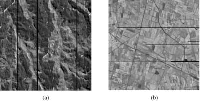
Figure 1: Simulated degraded scene: (a) Defect elements in a visible wavelength band (contrast enhanced), (b) Lost transmissions in a near-infrared band
Prior to the utilisation of affect imagery a reconstruction of the lost information is required. The detection of the concerned image lines is straightforward since faulty CCD elements can be eas-ily measured by observation of suitable targets with a homogenous spectral characteristic. This is of particular interest for partially degraded scanning elements. Lost transmissions on the other hand are picked up by the protocol of the receiving station. Therefore, for the remaining part of the paper it is assumed that the location of missing lines is known. Moreover, a differentiation between horizontal and vertical lines is not required since both cases are equivalent after rotat-ing the image. Henceforth for the sake of simplicity only vertical line artefacts are addressed and the problem is essentially considered as a one-dimensional reconstruction issue perpendicular to the artefact’s main principal orientation.
The actual restoration of the signal can be the source of undesirable errors in the further proc-essing chain and therefore has to be analysed carefully. The standard approach is the utilisation of linear and cubic interpolation kernels. However, the inherent low pass characteristic of these filters introduces blurring – especially for gaps that are wider than one pixel or in the presence of high spatial frequency content. Thus, this paper investigates two different techniques for the reconstruction that incorporate the nature of the data or an extended data region. Firstly, autore-gressive estimation is utilised and the issues of parameter estimation considered. Secondly, ra-dial basis functions are employed. Unlike the standard interpolation kernels this family of func-tions can make use of samples that are spatially further away from the actual missing data and hence models the underlying data characteristic. The inherently introduced artefacts are analysed for all different methods using multispectral imagery in the visible and near-infrared wavelength range obtained from SPOT. Although this satellite by itself does not suffer from the mentioned difficulties it is a good example due to its widespread choice of spectral bands. This paper is organised as follows: Section 2 provides an overview of the utilised reconstruction techniques and describes the different processing steps in detail. The actual results and their discussions are presented in Section 3. Finally, Section 4 concludes the paper.
2. RECONSTRUCTION MODELS
The actual reconstructions in this paper are performed for each band individually. For highly correlated bands the accuracy of the estimated missing data values could possibly be improved if the additional information of the other bands is utilised. However, generally this approach is only possible for the vertically oriented artefacts since the CCDs are independent from each other. But in case of transmission losses the information of the different bands is often interlaced and therefore a loss affects all bands.
2.1. Autoregressive (AR) Model
The name ‘autoregressive’ is derived from the concept of regressing an unknown value xj based on previous known values xi with i<j. In terms of the problem on hand the xi represent pixels left or right of the missing pixel while the xj corresponds to the defect CCD element. The estimation follows a linear model, i.e.
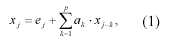
where e is the uncorrelated prediction error with zero mean and constant variance. The variable p determines the order of the model and hence the number of known values that are incorporated in the reconstruction of xj while the ak are weight coefficients with ak Î[-1,1]. If the gap is wider than one pixel, i.e. xj,…,xj+n are distorted, then an iterative approach is applied that estimates the unknown sequentially while utilising previous estimates as actual available values. Before the actual reconstruction can be performed, the order of the process as well as the coefficients have to be determined. Various algorithms are available for this purpose, however, the most promi-nent are the least square, Yule-Walker and Burg approach (Priestley, 1994; Rezek and Roberts, 1997). De Hoon et al. (1996) highly recommend the Burg method for AR parameter selection since usually Yule-Walker leads to poor parameter estimates and the least square method to un-stable models. Nevertheless all three techniques are used in this paper to provide a full compari-son and to reflect on their popularity.
The least square (LS) technique considers a simple regression between the predictor x and the dependent or response variable Y. Therefore the observation Y can be expressed by the random variable x and the unknown regression coefficients can be computed using a set of available observations while minimising the sum of squares of the residuals. The Yule-Walker technique is also known as the autocorrelation method. The Levinson-Durbin algorithm is used to solve the Yule-Walker equation, which explores the Toeplitz structure of the matrix to be inverted. This solves for the AR parameters more efficiently. Note that the ap-proach by Yule and Walker is expected to give the smallest prediction error of the three AR prediction models in this investigation.
The main idea behind the argumentation for the Burg algorithm is that knowledge of the auto-correlation coefficients is not sufficient to identify a process uniquely. Instead the coefficients are determined by a maximum entropy method by estimating the reflection coefficients at suc-cessive orders. The algorithm exhibits some bias in estimating the central frequencies of sine components. Moreover, higher order fits are affected by "splitting", a phenomenon where multi-ple peaks in the spectrum are generated instead of a single feature.
2.2. Radial Basis Functions
In this paper polyharmonic radial basis functions (RBF) are used for the reconstruction of the missing data. Basically, the image data describe multi-dimensional points that are approximated by the corresponding surface of the RBFs. For a given set of points xi with xi being a column vector in the multi-dimensional space, the RBF is described by
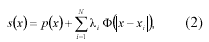
where p is a low-order polynomial, the li coefficients and F the actual basis function. Unlike other interpolation functions, e.g. linear, cubic and sinc, the RBF utilises all N available points. This is of particular interest, since the spatial extend of F is not limited as for the other listed in-terpolation kernels. The utilised function in this paper is the thin-plate spline F(r)=r 2 log(r). The major problem with respect to Equation (2) is to determine the coefficients of the polynom p and the li. Given the constraint
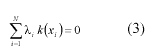
for all polynomial functions k with a degree smaller or equal to m, the problem can be solved by solving the corresponding linear system (Carr et al., 2001). For the actual realisation of the function fitting in this investigation, the special implementation of the RBF provided by the company aranz was chosen (ARANZ, 2003).
3. RECONSTRUCTION RESULTS AND EVALUATION
This section presents the results for the reconstruction using the two different approaches with various parameter settings. The performance comparisons among the different techniques are based on the data shown in Figure 1. Different gap widths were used to investigate the stability of the respective reconstructions. In this investigation the RMS errors between the reconstructed and actual values were used as a measure of accuracy.
3.1. Autoregressive Model
High-order AR models take more information from the neighbourhood around the missing data into account and use it to predict the missing pixel(s). This can be advantageous if a general trend has to be modelled. However, if data with high spatial frequency content have to be recon- structed then the approach generally cannot model the sudden changes. Table I shows the recon- struction performance of the Burg parameter estimation technique for different model orders and varying gap widths, i.e. the number of consecutively missing samples.
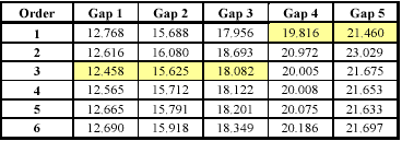
It can be seen from the table that the performance drops as the gap width increases which is due to the high spatial fidelity of the utilised near infrared band. It is worthwhile noting that consis-tently throughout all the conducted experiments the best performances for the Burg method with gaps less then four pixels wide were achieved with a third order model. Although the reasons for this phenomenon are not completely understood, it is reasonable to assume that the order pro-vides the best trade-off between estimation stability and incorporation of sudden changes. How-ever, with increasing gap width the lowest order is preferable.
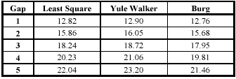
In the next experiment the performances of the three parameter estimation approaches were compared for a first order model. The results in Table II show that the Yule-Walker method per-formed the worst of all the three techniques, although not by a large margin. Note that the errors for the first three rows of the Burg approach can be further reduced by choosing a more suitable model order like shown in Table I.
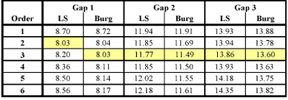
So far, the reconstruction process was considered as a reconstruction that starting from the left side estimates missing values towards the right side. While a change in orientation has no im-pact on the accuracy, the combination (mean) of both directions leads to a clear drop in the RMS error like indicated in Table III. Again, in almost all cases an optimum for the third order model can be observed.
3.2. Radial Basis Functions
The performance assessment of the RBF’s interpolation capabilities was conducted using three different approaches. Firstly, the functions were fitted directly to match the available data and hence the unknown parameters in Equation (2) were determined. Secondly, the fitting constraint was relaxed in terms of maximum tolerated difference between the actual and the used value. The motivation for this relaxation was to allow for noise in the image data and hence to incorpo-rate it in the reconstruction process. Thirdly, a special data reduction technique suggested by Carr et al. (2003) was utilised. The results for the three approaches are shown in Table IV.
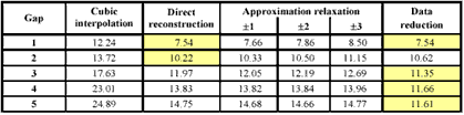
The approximation relaxation clearly decreases the reconstruction accuracy. This can be ex-plained by the very high SNR of the used SPOT data which renders the noise concerns towards zero. For small gap widths the performance of the direct reconstruction and the reduced utilisa-tion of available data points show equally good results. However, with an increased width the latter method evidently outperforms the first approach. The reasons are manifold but most im-portantly the reduction relaxes the requirement to incorporate all given data in the estimation process even if it is fairly unrelated. Last but not least the cubic interpolation as an example for a standard interpolation kernel was never able to achieve the best result.
4. CONCLUSIONS
The results show that the best reconstruction accuracy is provided by the radial basis functions. Depending on the gap width the preference is either with the direct reconstruction or the technique based on an actual sample reduction. However, radial basis functions come at a high cost in terms of required processing time. If this aspect is of importance and a slight less accurate performance can be tolerated then the mean over antipodal estimation directions using an auto-regressive model is preferable.
Future work will incorporate additionally available knowledge if only one of the bands is af-fected by the degradation. Hence, the estimation process can be stabilised.
REFERENCES
- ARANZ, 2003, http://www.aranz.com.
- Carr, J.C., Beatson, R.K., Cherrie, J.B., Mitchell, T.J., Fright, W.R., McCallum, B.C., Evans, T.R., 2001. Recon-struction and representation of 3D objects with radial basis functions. Proc. of the ACM Siggraph, pp. 67–76.
- Carr, J.C., Beatson, R.K., McCallum, B.C., Fright, W.R., McLennan, T.J., Mitchell, T.J., 2003. Smooth surface reconstruction from noisy range data. Proceedings of the ACM Graphite, pp. 119–126.
- De Hoon, M.J.L., Van der Hagen, T., Schoonewelle, H., Van Dam, H., 1996. Why Yule-Walker should not be used for autoregressive modelling. Annals of Nuclear Energy, 23, pp. 1219–1228.
- Priestley, M.B., 1994. Spectral Analysis and Time Series. Academic Press, London.
- Rezek, I.A., Roberts, S.J., 1997. Parametric model order estimation: A brief review. IEE Colloquium on the Use of Model Based Digital Signal Processing Techniques in the Analysis of Biomedical Signals, pp. 3/1–3/6.