| GISdevelopment.net ---> AARS ---> ACRS 2004 ---> New Generation Sensors and Applications: Digital Camera |
Remote Sensing of Turbidity
Mapping from Digital Camera Imagery
Sultan AlSultan
1 , H. S. Lim 2 , M. Z. MatJafri 3 , K.
Abdullah 3 and M. N. A. Bakar
4
1Dr., Al Sultan Environmental Research Center. Al Madina Rd., P.O.Box.
242 Riaydh Al Khabra, Al Qassim, Saudi Arabia.
Tel: +966504890977, Fax: +96663340366
Email: allssultan7@hotmail.com
2Student, 3 Assoc. Prof. Dr., 4 Dr., School of Physics,
University of Science Malaysia,
11800 Penang, Malaysia
Tel: +604-6533888, Fax: +604-6579150
Email: mjafri@usm.my, khirudd@usm.my
ABSTRACT
A complete set of normal digital camera data and ground-based measurements are used to test an algorithm for retrieval of turbidity distribution in the Prai Estuary, Penang, Malaysia. The main objective was to test the algorithm developed for total suspended solids (TSS) to be used for turbidity mapping. Empirical relationships are established between the raw digital number of the digital camera imagery bands and turbidity values obtained from field measurements. The digital imageries were captured from a light aircraft at a low altitude of 4400 feet. A bigger study area of coverage was obtained by using a mosaic image from eight digital images. Water samples locations were determined using a handheld GPS. The digital image was separated into three bands assigned as red, green and blue bands for multispectral algorithm calibration. The digital numbers were extracted corresponding to the ground-truth locations for each band and later used for the calibration of the developed algorithm. The efficiency of the present proposed algorithm, in comparison to other forms of algorithm, was also investigated. Based on the values of the correlation coefficient (R) and root-mean-square deviation (RMS), the proposed algorithm is considered superior. The calibrated TSS algorithm was used to generate the water quality map. The water quality image was geometrically corrected and the image was filtered to remove random noise. The generated map was colour-coded for visual interpretation. This preliminary result indicated that the previously developed algorithm for TSS was suitable used for turbidity mapping of the Prai Estuary, Penang, Malaysia.
1.0 INTRODUCTION
Water turbidity is an expression of the optical properties of water, which cause the light to be scattered and absorbed rather than transmitted in straight lines. It is therefore commonly regarded as the opposite of clarity. As water turbidity is mainly caused by the presence of suspended matter, turbidity measurement has often been used to calculate fluvial suspended sediment concentrations (Wass, et al., 1997).
Mostly, satellite data will be used for water quality monitoring, but the major disadvantage of satellite data is that, they cannot see through the clouds. Airborne digital camera imageries were selected in this present study because of several reasons. First was the airborne digital images provide higher spatial resolution data for mapping a small study area. Second was the airborne digital data acquisition can be carried out according to our planned surveys. The satellite observation times are fixed for a particulate study area. Third was the digital imagery offers many advantages over film-based cameras. There is a great saving of time because the data can be loaded directly to a computer for processing, as there is no need for film processing and scanning (Wicks, 2003). Remote sensing techniques have been widely used for water quality studies in coastal regions and in inland lakes (Ekstrand 1992, Ritchie et al.1990, Baban 1993, Dekker and Peters 1993, Dekker, et al., 2001, Forster et al. 1993, Allee and Johnson 1999, Koponen et al. 2002). In this study, algorithm was used to determine the turbidity distribution in the surface of seawater. The algorithm used in this study was developed based on the reflectance model for TSS. Various types of algorithms were tested and their accuracies were noted. Finally, the optimum algorithm was selected and used to generate a turbidity map over Prai Estuary, Penang, Malaysia.
2.0 STUDY ARAE AD DATA ACQUISITION
The location of the study area is in the vicinity of the Prai river estuary, Penang. It is situated between latitudes 5º 22’ N to 5º 24’ N and longitudes 100º 21’ E to 100º 23’ E (Figure 1). Images were taken during the flight between 9 a.m. to 11 a.m. on 1 September 2003. Turbidity readings were measured by using a handheld turbidity meter. Digital camera imagery was captured simultaneously during the acquisition of the water samples. Images were taken from an altitude of 4400 feet. Water samples locations were determined using a handheld GPS. In this study, airborne image was used instead of satellite imagery because of the difficulty in obtaining a cloud free satellite image in the equatorial region. River estuary is selected as the study area because of the TSS concentration is clearly differentiated.
Figure 1 The study area
3.0 WATER OPTICAL MODEL
A physical model relating radiance from the water column and the concentrations of the water quality constituents provides the most effective way for analysing remotely sensed data for water quality studies. Reflectance is particularly dependent on inherent optical properties: the absorption coefficient and the backscattering coefficient. The irradiance reflectance just below the water surface, R(l), is given by

Where l is the spectral wavelength, bb is the backscattering coefficient and a is the absorption coefficient (Kirk, 1984). The inherent optical properties are determined by the contents of the water. The contributions of the individual components to the overall properties are strictly additive (Gallegos and Correll, 1990).
For the case of two water quality components, i.e. chlorophyll, C, and suspended sediment, P, the simultaneous equations for the two channels can be expressed as
where bbw(i) is the backscattering coefficient of water, bbc*and bbp* are the specific backscattering coefficients of chlorophyll and sediment respectively, aw(i) is the absorption coefficient of water, ac*(i) and ap*(i) are the specific absorption coefficients of chlorophyll and sediment respectively (Gallie and Murtha, 1992).
4.0 REGRESSION ALGORITHM
Solving the above simultaneous equations (2a and 2b) for TSS concentration yields the series consisting of the terms R1 and R2

Where aj, j = 0, 1, 2, … are the functions of the coefficients in equation (3) which are to be determined empirically using multiple regression analysis. The algorithm can be extended to the three-band method for turbidity

And the coefficients ej, j = 0, 1, 2, … is then empirically determined.
5.0 DATA ANALYSIS AND RESULTS
Eight colour digital imageries of the Prai River Estuary were selected for algorithm calibration. The digital imageries were acquired in visible multispectral (3-bands: red, green and blue). The size of each raw airborne colour digital image of the Prai river estuary, Penang was 480 pixels by 720 lines. The eight images were mosaiced together for a bigger coverage area. The mosaic image was then separated into three bands, (red, green and blue bands) for multispectral analysis using PCI software package.
Digital number (DN) for each location of water sample was determined for each band. The locations were determined with reference to the selected ground control points (GCP) used in the image-to-map rectification method using the PCI software. Digital numbers were determined for each band using different window sizes, such as, 1 by 1, 3 by 3, 5 by 5, 7 by 7, 9 by 9 and 11 by 11. The DNs value extracted using the window sizes of 3 by 3 were used because the data produce higher correlation coefficient in the regression analysis. The plot of the relationship between the DN’s for each channel and the turbidity values is shown in Figure 2.
Figure 2 Graph of digital numbers versus turbidity
In this study, raw DN values were used as independent variables in our calibration regression analysis. Other forms of water quality algorithm were tested with the data set and their accuracies were compared with that of the proposed algorithm. For each regression model the correlation coefficient, R, and the root-mean-square deviation, RMS, were noted. Table 1 shows the comparative performance of the algorithm. The proposed algorithm produced higher correlation coefficient between the predicted and the measured turbidity values and lower RMS value compared to the other algorithms (Figure 3).
Figure 3 Relationship between measured and values predicted turbidity
* B1, B2 and B3 are the digital number for red, green and blue band respectively
Finally, a turbidity map was generated using the proposed algorithm. The generated map was colour-coded for visual interpretation and smoothing filter was applied to the image to remove the random noise (Figure 4).
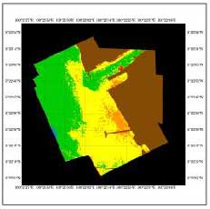
Figure 4 Map of turbidity near Prai River Estuary [Blue = (< 10 NTU), Green = (10-20) NTU, Orange = (20-30) NTU, yellow = (30-40) NTU, Red = (>40) NTU, Brown = Land and Black = area outside image]
6.0 CONCLUSION
The algorithm for the retrieval of turbidity using digital camera imagery was applied to the image of Prai River Estuary, Penang. The accuracy of the retrieval algorithm generated in this study was R = 0.9902 and RMS = 0.9616 NTU. This study shows that the digital camera is an effective tool for rapid determination of turbidity in Prai River Estuary, Penang.
ACKNOWLEDGEMENTS
This project was carried out using the Malaysia Government IRPA grant no.08-02-05-6011 and USM short term grant FPP2001/130. We would like to thank the technical staff who participated in this project. Thanks are extended to USM for support and encouragement.
REFERENCES
- Alle, R.J., and Johnson, J.E., 1999, Use of satellite imagery to estimate surface chlorophyll-a and Secchi disc depth of Bull Shoals, Arkansas, USA. International Journal of Remote Sensing, 20, 1057-1072.
- Baban, S.M., 1993, Detecting water quality parameters in the Norfolk Broads, U. K., using Landsat imagery. International Journal of Remote Sensing, 14, 1247-1267.
- Dekker, A.G., and Peters, S.W.M., 1993, The use of Thematic Mapper for the analysis of eutrophic lakes: a case study in the Netherlands. International Journal of Remote Sensing, 14, 799-821.
- Dekker, A. G., R.J. Vos, R. J. and Peters, S. W. M. 2001, Comparison of remote sensing data, model results and in situ data for total suspended matter TSM in the southern Frisian lakes. The Science of the Total Environment, 268, 197-214.
- Ekstrand, S., 1992, Landsat TM based quantification of chlorophyll-a during algae blooms in coastal waters. International Journal of Remote Sensing, 13, 1913-1926.
- Forster, B.C., Xingwei, I.S., and Baide, X., 1993, Remote sensing of water quality parameters using landsat TM. International Journal of Remote Sensing, 14, 2759-2771.
- Gallegos, C. L., and Correld. L., 1990, Modeling spectral diffuse attenuation, absorption and scattering coefficients in a turbid estuary. Limnology and Oceanography, 35, 1486-1502.
- Gallie, E. A., and Murtha, P. A., 1992, Specific absorption and backscattering spectra for suspended minerals and chlorophyll-a in Chilko Lake, British Columbia. Remote Sensing of Environment, 39, 103-118.
- Kirk, J. T. O., 1984, Dependence of relationship between inherent and apparent optical properties of water on solar altitude. Limnology and Oceanography, 29, 350-356.
- Koponen, S., Pulliainen, J., Kallio, K., and Hallikainen, M., 2002, Lake water quality classification with airborne hyperspectral spectrometer and simulated MERIS data. Remote Sensing of Environment, 79, 51-59.
- Ritchie, C. J., Cooper, C. M., and Yong, Q. J., 1987, Using Landsat Multispectral Scanner data to estimate suspended sediments in Moon Lake, Missisippi. Remote Sensing of Environment, 23, 65- 81.
- Waldron, M. C., Steeves, P. A., and Finn, J. T., 2001, Use of thematic mapper imagery to assess water quality, trophic state, and macrophyte distributions in Massachusetts lakes. Water-Resources Investigations Report 01-4016.
- Wass, P. D., Marks, S. D., Finch, J. W., Leeks, G. J. L. and Ingram, J. K. 1997, Monitoring and preliminary interpretation of in-river turbidity and remote sensed imagery for suspended sediment transport studies in the Humber catchment, The Science Of The Total Environment, 194&195, 263- 283.
- Wicks, D. E., 2003, Emerging trends in mapping using LIDAR and Digital Camera Systems. Proceeding of the Map Asia 2003, Photogrammetry and LIDAR