| GISdevelopment.net ---> AARS ---> ACRS 2004 ---> New Generation Sensors and Applications: Line Scanner |
Three Dimensional Positioning
for Airborne Three-Line-Scanner Images
Liang-Chien Chen, Shih-Che
Lin, Tee-Ann Teo
Center for Space and Remote Sensing Research
National Center University
Chung-Li, TAIWAN
Tel: +886-3-4227151 ext 57622, 57623 Fax: +886-3-4255535
Email: lcchen@csrsr.ncu.edu.tw, 92322090@cc.ncu.edu.tw, ann@csrsr.ncu.edu.tw
Center for Space and Remote Sensing Research
National Center University
Chung-Li, TAIWAN
Tel: +886-3-4227151 ext 57622, 57623 Fax: +886-3-4255535
Email: lcchen@csrsr.ncu.edu.tw, 92322090@cc.ncu.edu.tw, ann@csrsr.ncu.edu.tw
Abstract
The purpose of this investigation is to perform 3-D positioning using three-line-scanner Level 1 images. Three major steps are included: (1) definition of the geometry of the triplet, (2) calculation of orientation parameters, and (3) space intersection. In the first step, the exterior orientation parameters are expressed as low-order polynomials with respect to time. The additional parameters are used to represent image coordinates including forward and backward images. Then, the orientation parameters are calculated by space resection. Finally, the results are checked by space intersection. A set of ADS40 data covering the area of Waldkirch of Switzerland is used for validation. The experimental results indicate that the proposed method is simple and yet may reach high accuracy.
1. INTRODUCTION
Airborne three-line-scanner images have the merits of high spatial and spectral resolutions, and excellent converging geometry. Thus, the images have become an important data source in environmental remote sensing and GIS application. In order to extract 3D information from the images, orientation modeling is a prerequisite. The bundle adjustment is often used to calculate the dynamic orientation parameters with respect of time for three images (Shibasaki et al, 2003). The method might contain local systematic errors for the data with high dynamics, thus, a least squares filtering that performs orbit collocation is preferable.
Before calculation of bundle adjustment, the imaging geometry has to be constructed. At the initial stage of this investigation, we perform the space resection to calculate the orientation parameters. Then the orientation parameters may be used in three-dimensional positioning by intersecting three rays for conjugate points.
In the space resection, we compare two different methods. The first one is the scene dependent approach that means each image has its own orientation parameters. This simplified method assumes that the three images have no geometric constraints. The second method considers that the three images have the same orbit and attitude parameters. The CCD distances between forward, nadir, and backward are pre-calculated, and we then use those values to connect three images by including additional parameters.
The purpose of this investigation is to perform three-dimensional positioning using three-line-scanner Level 1 images. Different from the raw data, the Level 1 images have been preliminarily rectified using GPS and INS data. The distortions in the scenes of Level 0, caused by the motion of the sensor, are mostly removed by this rectification (L. Hinsken, et al 2002). Therefore, the images include small tilt displacements. The central tasks include: (1) definition of the geometry of the triplet, (2) calculation of orientation parameters, and (3) calculation the ground points by space intersection. The workflow of investigation is in figure1.
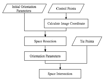
Figure 1. Workflow of the investigation
2. ORBIT ADJUSTMENT
The major works are the calculation of the position parameters and attitude data, followed by the three-dimension positioning on ground. Two steps are included in this stage. The first step is to define the imaging geometry of triplet. Then, the orientation parameters are calculated by space resection using the triplets. The orientation parameters are expressed as low order polynomials with respect of time (Gruen & Zhang, 2003). Finally, the conjugate points are used for three-dimensional positioning by space intersection.
2.1 Definition of parameters
The orientation parameters , ö , ê , X c , Y c , Z c ) are expressed as second-order polynomials function with respect to time .The dynamics is shown in eq.1.
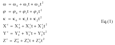
Then, the collinearity equations are employed to relate the image coordinates(x, y) and the object coordinates(X, Y, Z). Because three different images are used, the image coordinates have to be defined with new parameters. The modified collinearity condition equations are used as shown in eq.2. The x is a constant number, which are calculated by the focal length and the look angle. The scale number is used to correct the image coordinate error in y direction. The . x and . y are additional parameters for the compensation of systematic errors.
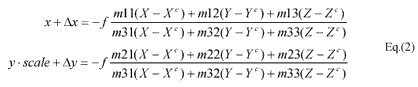
In addition to the 18 unknown orientation parameters, we include the additional parameters (x, . y, scale) to compensate image coordinate for forward and backward images. The geometric relation of the triplet images is shown in figure2.
Figure 2. Geometric relation of the triplet
2.2 Calculation of orientation parameters
We calculate orientation parameters and additional parameters by space resection. A least squares adjustment is performed to determine the orientation parameters.
2.3 Space intersection
When the orientation parameters are determined, we use the tie points in three images to calculate the ground coordinates. Then, error ellipses are calculated to analyze the precision.
3. EXPERIMENT RESULTS
A set of ADS40 Level 1 data covering the area of Waldkirch of Switzerland is used. The related ADS40 parameters are shown in table 1. The images have about 0.2m ground resolution. The images are shown in figure3. In test area, 11 ground control points are employed for the adjustment, and 40 conjugate points for precision check. The experiment includes the comparisons of (a) independent orientation modeling for each strip, and (b) unified orientation parameters for the triplet.
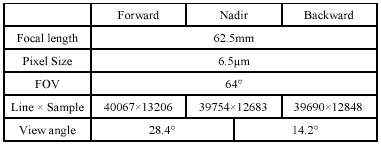
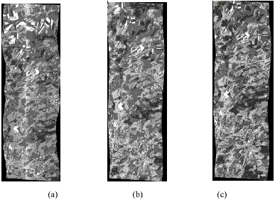
Figure 3. Test area of ADS40 imagery .cADS40 Image Copyright 2002 Leica (a) Forward (b)nadir (c)backward
3.1 Results of Independent Approach
Because limited numbers of GCPs are available, additional parameters are not considered in this test. After the adjustment of independent orientation modeling for each strip, the RMSEs are about 1.5 pixels both in X, and Y directions for the GCPs when using 11 GCPs. The residual vectors are illustrated in figure 4. In the figure, red, green, and blue vectors are for forward, nadir and backward, respectively. Notice that the RMSEs are not reliable due to its low degree of freedom when 22 equations were used to solve 18 unknowns. Thus, we manually measure the conjugate points for evaluation by space intersection. The error ellipses in X-Y direction and the error bars in z direction are shown in figure 5 (a) and figure 5 (b), respectively. The RMSE of semi-major axis is 0.9m. The standard error in Z-direction is 2m.
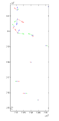
Figure 4. Residual vectors of GCPs
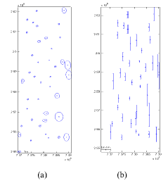
Figure 5. Error ellipses (a) Ellipses in X-Y direction (b) Error bar in Z direction
3.2 Results of Unified Approach
The second test is the unified approach for the triplet. In this case, 66 equations were formulated to solve 24 unknowns. Thus, much higher degree of freedom is available than in the previous case. The RMSEs are about 2.5 pixels for the GCPs when using 11 GCPs. The residual vectors are illustrated in figure 6. The color code in figure 6 is identical to figure 4. The error ellipses in X-Y direction and the error bars in Z direction are shown in figure 7 (a) and figure 7 (b), respectively. The RMSE of semi-major axis is 0.4m. The standard error in Z-direction is 0.8m.
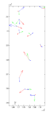
Figure 6. Residual vectors of GCPs
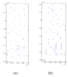
Figure 7. Error ellipses (a) Ellipses in X-Y direction (b) Error bar in Z direction
It is observed that the unified approach is better than the independent approach. However, there are still some local systematic errors. Thus, the bundle adjustment with least squares filtering would be needed for higher precision.
4. CONCLUSIONS
This objective of this investigation is the three-dimensional positioning for three-line-scanner imagery. The first step of the proposed scheme is to determine the orientation parameters. Then, we use the space intersection to evaluate the three-dimensional positioning. Experimental results indicate that the unified approach is significantly better than the independent approach. The unified approach may reach the errors of 0.3m, 0.2m, and 0.7m for X, Y, Z axes, respectively when 11 GCPs were employed. In the future, the bundle adjustment and least squares filtering would be included for higher accuracy.
REFERENCE
- Baltsavias, E. & M. Pateraki, 2002, “Adaptive multi-image matching algorithm for the airborne digital sensor ADS40”, Map Asia 20002, Asian Conference on GIS, GPS, Aerial Photography and Remote Sensing.
- Gruen, A., & L. Zhang, 2003, “Sensor modeling for aerial mobile mapping with Three-Line-Scanner Imagery”, International Archives of Photogrammetry and Remote Sensing, Vol.34, part II.
- Hinsken, L. , S. Miller, U. Tempelmann, R. Uebbing, S. Walker , 2002,“Triangulation of LH systems’ ADS40 Imagery Using Orima GPS/IMU”, Proceedings of ISPRS Commission III Symposium, PCV'02, 9-13 September, Graz, Austria.
- Shibasaki, R., S. Murai, T. Chen, 2003, “Development and Calibration of the Airborne Three-Line Scanner Imaging System”, PE&RS Vol.69, No.1.January, pp. 71-78