| GISdevelopment.net ---> AARS ---> ACRS 2002 ---> Photogrammetry |
Finite Element Method for
Rectification of Architectural Heritage Images of National Importance
Kamal Jain
Member CIPA TG-2
Department of Civil Engineering,
Indian Institute of Technology,
Roorkee – 247667, Uttranchal State, India
Email: kjainfce@iitr.ac.in
P.K. Garg
Member CIPA TG-2
Kamal Jain
Member CIPA TG-2
Department of Civil Engineering,
Indian Institute of Technology,
Roorkee – 247667, Uttranchal State, India
Email: kjainfce@iitr.ac.in
P.K. Garg
Member CIPA TG-2
Abstract
Photogrammetry has many advantages as a technique for the acquisition of facade information of the cultural heritage. However, the photogrammetric process to extract facade information from stereo images is often considered to be too labor-intensive and complicated. As a result of this consideration, existing images are often not used for a photogrammetric documentation of the object.
Photogrammetric single image techniques, like the generation of rectified images and orthoimages are well suited for use in architecture and monument preservation. They combine true scale geometric measurements with full image information under quite inexpensive production costs. Especially in the field of architectural orthoimage generation, the combination of image processing with photogrammetric systems provides new solutions.
An image rectification methodology for the reconstruction of destroyed historical buildings using single-view photographs has been presented in this work. Certain feature-oriented properties, like linearity, parallelism, perpendicularity, symmetry etc., of these historical buildings have been used in addition to the information extracted from the images. It has been assumed that neither camera information nor stereo views are available.
The method has been compared with the prevalent methods based on Projective, Polynomial and Affine transformation. The proposed method first generates image of equivalent grids from an available one using perspective geometry. Thereby extending the control throughout the image. Each image grid is then mapped on to the actual grid using finite element interpolation function. Since mapping is done taking the grid points as node points, the method automatically does mosaicking of different pieces.
1. Introduction
Digital rectification with digital image utilizes a personal computer with analytical photogrammetry solution. There are two classes of rectification approaches: the parametric and the non-parametric approaches. Whereas for the parametric approach, the knowledge of the interior and exterior orientation parameters is required, non-parametric approach requires more number of control points.
The parametric approach uses a reverse ray tracing to determine the grey values for all pixel positions in the rectified image. Re-sampling of the grey values requires the position of corresponding position in the distorted image. This can be calculated by the collinearity equations using interior and exterior orientation parameters and the position of the corresponding point in the object coordinate system. The interior orientation may be known from a calibration protocol of the image and a measurement of fiducial marks or a reseau. The exterior orientation parameters can be calculated by a resection in space using at least three control points or a bundle adjustment. Interior and exterior orientation parameters can also be estimated together within a spatial resection. In this case, the spatial distribution of the control points plays an important role in order to obtain the accurate results.
In case of non-parametric approaches, a planar coordinate transformation between the matrices of the distorted and the rectified image is used. The object coordinates of the control points have to be first reduced to 2D-coordinates on the projection surface.
In both the methods, least square adjustment is used, if number of control points are more than the required points. Further, in these methods control points should be distributed all over the image in a systematic way, so that the major portion of the image lies inside the control points, as these methods propagate errors in extrapolation. Generally, control points are available with varying accuracy, and therefore with the help of least square adjustment, error is distributed in all the control points even with better accuracy.
The finite element method was originally developed for structural analysis, but the general nature of the theory on which it is based, has made its application possible in other fields of engineering also. In finite element method, it is possible to express the displacements of any point within the element in terms of its nodal displacements using the shape functions. In other words, if a rectangular image is transformed into any arbitrary quadrilateral shape, the new pixel coordinates for each pixel in the parent image can be computed, if its nodal displacements are known.
Common Analytical Rectification Methods
1. Affine Transformation: assumes that there exist two different scales along both the directions X and Y.
This has six unknown parameter, a’s and the b’s, although the real unknowns are only five, viz., Sx , S
2. Polynomial Transformation: In view of the propagated error or orderly and systematic deformation often a polynomial transformation is found to be convenient.
3. Projective Transformation: It uses following equations:
This indicates that the projectivity between two planes is uniquely determined if a total of eight coefficients are known. This requires at least four points whose both X and Y coordinates in both the spaces are known. (Theodoropoulou)
The Finite Element Concept
In finite element methods, the variation of displacements etc., in the element is expressed as a function of its nodal values, which is known as displacement function, or interpolation function or shape function. The representation of geometry in terms of (non linear) shape functions can be considered as a mapping procedure, which transforms a regular shape, like a straight-sided rectangle in local coordinate system into a distorted shape, like a curved sided rectangle in global cartesian coordinate system. A displacement function is commonly assumed in a polynomial form, and practical considerations limit the number of terms that can be retained in the polynomial. An exact solution for displacement u (x), is approximated by various degree polynomials of the general form, as given below (Reddy, 1985):
n(x)=a1+a2x+a3x2+a4x3.................an+1xn (4)
In Eq. 4, x is one-dimensional variable and ai’s are (4) coefficients. The greater the number of terms included in the approximation, the more closely the exact solution is represented (obviously, this last statement does not apply to the case wherein the exact solution is a polynomial of some finite order ‘m’. Here terms in excess of ‘m’ do not improve the representation).
Consider a square parametric patch in unit coordinate space, 0< x, h<1. A linear parametric curve has the following form (Rao, 1982)–
L1 = 1-x 5(a)
L2 = x 5(b)
x(x ) = (1-x )x1 + x x2 (6)
In two dimensions, the shape functions is as follows (Fig 1):
L1 = (1-x )(1-h ) 7(a)
L2 = x (1-h ) 7(b)
L3 = xh 7(c)
L4 = (1-x ) 7(d)
and x(x , h) = Li (x, h)xi (8a)
y(x , h ) = Li (x, h )yi (8b)
Fig. 1-Linear parent elements and their transformations
This is called bilinear parametric Lagrangian quadrilateral. Since (xi, yi) are arbitrary, the patch is a straight-sided quadrilateral in physical space, even though it is always square in its so-called parent form. The above parametric form is linear at any edge but is an incomplete quadratic parametric on the interior of the surface. It is missing the x2 and h2 terms needed for a complete quadratic.
Methodology Developed
In the present work a methodology is proposed to divide the image into number of pieces using its perspective geometry provided by a four control points. Nodal points/pass points are also generated in each piece. Each piece is independently rectified using finite element interpolating functions.
Since the proposed method will do piece wise rectification, hence the image is expected to be exactly fitted with control points. The method generates nodal points in all over the image area on the basis of its perspective geometry; therefore, the accuracy is not affected in extrapolation.
- Original image of an oblique photograph is displayed on screen. (Fig.2)
- The four control points 1,2,3 & 4 of a trapezoid are selected on the displayed photograph using a cursor. Trapezoid represents a square on the target.
- The trapezoids 1,2,3,4 is extended to 1,2,6,5; 2,6,13,7; 2,13,14,3; 3,14,11,10; 3,10,9,4; 4,9,12,16; 4,16,15,1 & 1,15,8,5 etc.
- Thus, the whole photograph is divided into number of trapezoids. Each trapezoid represents a virtual image of a square that is a replica of the square 1, 2, 3, 4, on the ground (Fig. 3).
- Method of Inverse mapping using Finite Element is used to map each trapezoid into a square at its appropriate position in the rectified image.
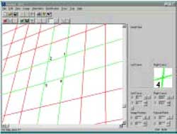
Fig 2

Fig 3
Comparison With Other Methods
In order to compare the proposed method with other methods of rectification, tilted photograph of a façade of a monument as shown in Fig. 4 has been taken for rectification. Projective transformation, affine transformation and polynomial of order 2 along with the proposed method have been used. The photograph has been rectified in two ways, as explained below:
- Control points are covering the maximum area on photograph.
- Control points are inside the image covering only about 20% of the photograph.
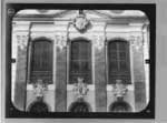 Fig 4 - Original tilted photograph |
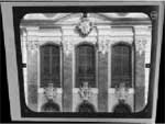 Fig. 5 - Rectified photograph using projective transformation |
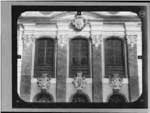 Fig. 6 - Rectified photograph using affine transformation |
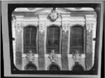 Fig. 7 - Rectified photograph using polynomial of order 2 |
Case II: The control points are selected on the middle window panel of Fig.4. Fig. 8, Fig. 9 & Fig. 10 show the transformed images using projective transformation, affine tranformation and polynomial of order 2 respectively. In Fig. 8, the middle window panels have become straight but the outer pillars are still converging. In Fig. 9, all the pillars are converging and in Fig. 10 the pillars are not only converging but are also deformed. Therefore, it is clear that affine transformation and polynomial of order 2 do not produce accurate results after the rectification of images. Fig. 11 shows the rectified image using the proposed method. Here all the pillars appear vertical after rectification.
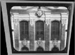 Fig. 8 - Rectified photograph using projective transformation |
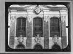 Fig. 9 - Rectified photograph using affine transformation |
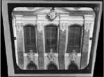 Fig. 10 - Rectified photograph using polynomial of order 2 |
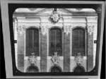 Fig 11 - Rectified photograph using proposed method |
Conclusions
The proposed method provides better accuracy than the normally used analytical methods e.g. Projective Transformation, Affine Transformation and polynomial of different order. Normal analytical methods work well in interpolation but Finite Element divides the entire image into number of pieces. The rectification is done piece by piece. Hence, it controls the error in extrapolation also. Finite Element Method uses inverse mapping. Therefore, resampling of rectified image is not required. The errors occurred due to resampling are also avoided. The max. shift observed on the extreme grid points is limited to 2.5 pixel. The rmse is found as 1.8 pixels.
References
- Rao, S. S., The Finite Element Methods in Engineering, Pergamon Press, Oxford, England, pp. 228-234. 1982
- Reddy, J.N., An Introduction to the Finite Element Method, Mc Graw-Hill Book Company, New York. pp 194-254. 1985
- Theodoropoulou Iliana, Single Image Photogrammetry with Analytical Surfaces A review prepared for the CIPA Task Group 2 "Single Images in Conservation"