| GISdevelopment.net ---> AARS ---> ACRS 2002 ---> Photogrammetry |
Image Orientation by Fitting
Line Segments to Edge Pixels
Sendo Wang
Ph.D. Candidate
Department of Surveying Engineering, National Cheng Kung University
No. 1, University Road, Tainan 70101, CHINA TAIPEI, R.O.C.
E-Mail: mailto:sendo@sv.n%20cku.edu.tw
TEL: +886-6-2370876 ext.839, 835
Yi-Hsing Tseng
Associate Professor
No. 1, University Road, Tainan 70101, CHINA TAIPEI, R.O.C.
E-Mail: tseng@mail.ncku.edu.tw
FAX: +886-6-2375764
Abstract
A new approach to recovering image exterior orientation for photogrammetry by Least-Squares Model-Image Fitting (LSMIF) is proposed in this paper. Instead of solving the space resection of well- distributed control points, the proposed method uses line segments as control lines. The control line segments are projected onto the image based on the approximate image orientation, and fit to the extracted edge pixels by varying the orientation parameters. The image orientation is determined when the projected line segments optimally fit to edge pixels. This paper describes the objective function and the adjustment process of the proposed fitting algorithm. Two examples of determining image orientation for a close-range and an aerial image respectively with the proposed method will be demonstrated.
1.Introduction
Recovering the image orientation refers to restoring the geometric relation between the sensor and the object at the moment of taking photograph, which is the fundamental task of a photogrammetric, remote sensing or computer vision application. The space resection is traditionally applied to solve the orientation for a single image with the measurements of the image coordinates of the control points. This point-based technique has been successfully applied in many analytical or digital photogrammetric applications. However, manual measurements is required to apply the techniques. The higher-level features, such as lines, planes, or object models, are not only easier to be found in the natural environment but also more meaningful than the point features. Therefore, a substantial research on using higher-level features has been carried out both in photogrammetry and computer vision domains in the last two decades (Haralick and Cho, 1984; Mulawa, 1989; Liu et al., 1990; Jaw, 1999; Smith and Park, 2000).
The idea of using straight lines as control elements for photogrammetry was initiated by Mulawa and Mikhail (1988), in which the space resection are re- formulated based on 3D straight-line equations. Since the line equation can be determined by measuring any two points on it, measuring three lines that are not on the same plane will be able to determine the photo’s orientation. Although it requires more measurements than point- based methods, t he measured points on overlapped photos do not have to be identical, which reduces the difficulty of image interpretation and avoids the point-matching problem. This concept has been expanded to using various types of line segments, even the free form curves, by many researches (Buchanan, 1992; Zielinski, 1992; Petsa and Patias , 1994 ; Schwermann, 1994; Forkert, 1996; Schenk, 1999; Zalmanson, 2000) . However, manual measurements of projected line segments on the image are still required.
Ebner and Strunz (1988) proposed another approach to recovering the exterior orientation by Digital Elevation Model (DEM) grid patches. Measuring more than three points on the same patch will provide a set of plane equations. The exterior orientation can be determined when all of the measured planes fit to the corresponding control surfaces by minimizing their Z-axis differences. This method is not suitable for the surfaces are near vertical. Jaw (1999) improved the method by minimizing the difference along the normal direction of the surface instead of the Z- axis. These area-based methods are suitable while the DEM has been known or can be derived from other sources like Light Detecting And Ranging (LiDAR) or Synthetic Aperture Radar (SAR) data, but it requires more computations and still needs manual measurements.
In this research, the building model is adopted as the control element for solving image exterior orientation. The wire -frame model of the known building is decomposed into 3D line segments and projected onto the image based on the approximate orientation. The optimal image orientation is solved by varying orientation parameters to achieve the optimal fit between projected line segments and extracted edge pixels on the image. This solution applies least-squares fitting algorithm and does not require any image measurement.
The general idea of the least-squares fitting is to minimize the squares summation of the distances from each edge pixel to the corresponding projected line segment. The fitting algorithm starts from a given first approximation of image orientation and solves for the correction of image orientation iteratively to find the optimal fitting. A buffer of each projected line segment is provided to determine that each pixel is corresponding to which line segm ent. It is assumed that the interior orientation of the camera is known, so that the unknown parameters are the coordinates of the perspective center and 3 rotation angles. The study cases include a close-range image pair and an aerial photo. The accuracy of image orientation by fitting line segments to edge pixels will be analyzed.
2. Orientation Recovery using Linear Features
Recovering the image orientation refers to restoring the geometric relation between the sensor and the object at the moment of taking photograph, which is the fundamental task of the photogrammetric, remote sensing or computer vision applications. It is usually divided into two parts as consideration, the interior orientation and the exterior orientation. The exterior orientation refe rs to the geometric relation of the sensor in the object space, which can be represented by parameters such as the object coordinates (X0, Y0, Z0) of the perspective center, and the rotation angles of the sensor. The exterior orientation parameters can be solved by space resection for single photo, independent model adjustment or bundle adjustment for multiple photos. These traditional techniques are based on measuring points on the images and corresponding them to their 3D coordinates in object space. However, the point- based methods are difficult to be automated due to the lack of robust image interpretation and intelligent point- matching algorithm. The tremendous points-measuring work is still remains for human.
The linear features are easily to be identified in the natural environment, such as roads, walls, or building edges, which gives them more potential than the point features. Usin g linear features for recovering image orientation is based on the constraint that, a 3D line as any vector connecting the perspective center with an arbitrary point on the 3D line must lie in the plane defined by the perspective center and the correspondi ng 2D lines (Zalmanson, 2000). If the line equations of a 3D line is known from existing maps, building models, or GIS data, then measuring any two points on the corresponding 2D line will provide a set of constraint equations, which is similar to the collinear equations formed by control points. Although the measuring points do not have to be identical on overlapped images, it still requires manual identification and measurement.
In this research, the interior orientation is derived from the camera calibration before the photogrammetric task. Our major concern is to recovering the exterior orientation by fitting projected line segments to extracted edge pixels without any manual measurements. Many linear features in the environment, such as a section of road or a piece of wall, could provide the 3D control line segments. The existing Constructive Solid Geometry (CSG) building model is a better source, for several line segments can be composed of their vertices simultaneously. These line segments are then projected onto the image with approximate exterior orientation for the fitting purpose. On the other hand, the edge pixels are extracted automatically by using edge- detecting algorithms. The image orientation now can be determined by varying the exterior orientation parameters so that the extracted pixels are optimally fit to the projected line segments. Least-squares Model-image Fitting (LSMIF) is applied to achieve optimal fitting, the details will be described in the next chapter. Figure 1 illustrates the process.

3. Least-Squaresmodel-Image Fitting
All of the edges of the CSG building model are projected onto the photo by collinear equations with approximate exterior orientation parameters for the fitting purpose. There are two ways to get approximate exterior orientation parameters: (1) given from other sources, for example, the Inertial Measuring Unit (IMU) and Global Positioning Sys tem (GPS); (2) calculated by manually adjusting the projected model to fit its image approximately. After the projection, all of the edges are evaluated by self- occlusion test to determine if it is visible. Take the box-like building model for example, the re are maximally 9 edges visible on a photo and others are occluded by the model itself. Even the edge passed the self-occlusion test, it is still possible occluded by other objects, like trees, building, or shadow. Unfortunately, the situation is difficul t to be detected automatically due to the lack of an efficient image interpretation algorithm, therefore, it still requires manually interaction to remove the fully occluded line segments.
The edge pixels must be extracted from the image so the corresponding line segment can be fit. There are many well-developed edge-detecting algorithms, such as Laplacian of Gaussian (LoG) and Canny operator. After comparing their performances for extracting building edges, we chooseChio’s (2001) program RSIPS. It is based on the algorithm of the polymorphicFeature EXtraction module (FEX) developed by Förstner and Fuchs (Förstner, 1994; Fuchs, 1995; Fuchs and Förstner, 1995) , which can extract interest points, edges, and regions simultaneously. The extracted edge pixels are then transformed into photo coordinate system with calibratedinterior orientation parameters.
To reduce the influence of the irrelevant pixels, a buffer range along each of the projected line segment is selected. The extracted edge pixels that are inside the buffer are considered as the real edge image and used for the least-squares fitting, others are ignored. Figure 2 shows one of the projected line segment and its buffer range. The selection of buffer range is critical to the fitting. Because a wide buffer range may include the irrelevantpixels and result in fitting incorrectly, while the narrow buffer range may miss the correct edge image and result in the failure.
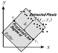
Figure 2. The selected buffer of a projected
That the fitting condition we are looking for is the projected line segment exactly falls on most of the edgepixels in the image. It means that the distancedi form extracted pixelTi to the projected line segment v1v2is considered as a discrepancy and is expected to be zero. Therefore, the objective of the fitting function is to minimize the distance between the extracted edge pixels Ti and the projectedline segmentv1v2. The projected edge is composed of the projected vertices v1 (x1, y1) and v2 (x2, y2). Suppose there is an extracted edge pixel Ti (xti, yti) located inside the buffer, the distance di from the point Ti to the edge v1 v2 can be formulated as the following equation:
where i is the index of extracted edge pixel.
The photo coordinates v1 (x1, y1) and v2 (x2, y2) are functions of the exterior orientation parameters. Every extracted edge pixel in the buffer may form an objective function as Equation ( 1). Since di represents the discrepancy between model and image, the objective of fitting is to minimize the squares sum of the distances:

Appling the least-squares adjustment to the fitting function, the distance di is considered as the residual errors vi. Therefore, Equation (1) should be rewritten as follows:

Equation (3) is nonlinear and the unknowns cannot be calculated directly. In order to solve the unknowns using Newton-Rapheson method, Equation (3) should be differentiated with respect to the unknown parameter. Then, it may be expressedin the linearized form as:

In Equation (4), Fi0 is the approximation of the function Fi evaluated by the given initial value of the 6 unknowns – the exterior orientation parameters. The coefficients
 etc., are the partial derivatives of
Fi with respect to the indicated unknowns evaluated at the
initial approximations. The unknown parameters ÄX0,Ä
Y0,ÄZ0,Ä , Ä,Ä are increments of theexterior
orientation parameters applied to the initial approximations.
etc., are the partial derivatives of
Fi with respect to the indicated unknowns evaluated at the
initial approximations. The unknown parameters ÄX0,Ä
Y0,ÄZ0,Ä , Ä,Ä are increments of theexterior
orientation parameters applied to the initial approximations. Each extracted edge pixel will contribute such an equation for the corresponding projectedline segment. Therefore, a visible edge may have a group of observation equations. All of these equations can be summarized and expressed by the matrix form:V=AX- L, where A is the matrix of partial derivatives and X is the matrix of increments ofexterior orientation parameters. Once an edge pixel is added, it adds a row to matrix A, V, and L. It is easy to solve the matrix X by the matrix operation: X=(ATPA)- 1ATPL. If the weights of all unknowns are assumed equal, P is an identical matrix. If any element of matrix X does not meet the requirement, adding the increments on the initial parameters to regenerate the new matrix A and L, then implement the adjustment again. The iteration continues until the increments converge below the thresholds or diverge beyond the limits. When the iteration converges,all ofthe line segments are fit to theedge pixels and theimage orientation parameters are determined.
4. Experiments
The proposed method should be able to be applied both in close- range and aerial photogrammetry. The first experiment is designed to test the performance of the proposed method in close- range photogrammetry. We use the Fujifilm S1 Pro digital camera, which has a 3040*2016 Super CCD array, to take all of the close-range images. The focal length, shutter speed, and the aperture size remains the same as it is calibrated, so the interior orientation parameters from calibration are adopted directly. The second experiment is designed to test the ability while applying to aerial photographs. The photograph is taken by Zeiss LMK Aerial Survey Camera at 1600m height with focal length 305.11mm lens, as a result, the average photo scale is about 1:5000. The photograph is then digitized as digital image by photogrammetric scanner in 25m resolution.
4.1 Tests for Close-range Images
To test the performance of the proposed method, we select a building in NCKU campus and take two photos of it, as Figure 3. The 3D coordinates of the building vertices were measured in previous aerial photogrammetric job, and are used to construct the 3D line segments. After the fitting, the 3D Line segments are projected onto the image with the optimal exterior orientation, and the parameters are compared to the space resection results that use the vertices as control points. The maximum difference of perspective center position is less than 0.15m while the minimum is 0.02m. The maximum difference of rotation angle is less than 0.19° while the minimum is 0.006°. Table 1 lists the optimal exterior orientation parameters after LSMIF and their differences to space resection results. Figure 4 shows the extracted edge pixels and the final projection of the 3D line segments after LSMIF.
Table 1. The optimal exterior orientation parameters of LSMIF and the differences compared to space resection.
| Exterior Orientation Parameters | Left Image | Right Image | ||||
| LSMIF | Space Resection | Differences | LSMIF | Space Resection | Differences | |
| X0 (m) | 169312.111 | 169312.003 | 0.108 | 169310.694 | 169310.660 | 0.034 |
| Y0 (m) | 2544907.962 | 2544907.982 | -0.020 | 2544891.166 | 2544891.237 | -0.071 |
| Z0 (m) | 52.592 | 52.721 | -0.129 | 52.640 | 52.699 | -0.054 |
| (degree) | -54.871687 | -54.710991 | -0.160696 | -40.087423 | -40.077875 | -0.009548 |
| (degree) | -50.897328 | -50.891053 | -0.006275 | -59.595929 | -59.545863 | -0.050066 |
| (degree) | -149.302008 | -149.120890 | -0.181118 | -132.716189 | -132.661186 | -0.055003 |
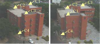
Figure 3. The original close-range images of the building.
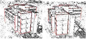
Figure 4. The extracted edge pixels and the optimal projected line segments.
There is an alternative to evaluate the accuracy of LSMIF, by comparing the check points coordinates. The 3D coordinates of the checkpoints, C1, C2, C3, and C4 shown in Figure 3 has been measured from the previous aerial photogrammetric work. Since we have a stereo pair and the orientation are recovered by LSMIF, the 3D coordinates of the check points can be calculated using intersection. Comparing the calculated coordinates to their previous coordinates will give a clear picture of the LSMIF accuracy. Table 2 lists these coordinates and their differences. The maximum difference is 0.193m on X- coordinate and –0.128m on Y- coordinate of C2, while other coordinates differences are between ±0.06m. It shows that the accuracy has been close to the stereo measuring in aerial photogrammetry and, therefore, is acceptable.
Table 2. Check points coordinates comparison.
| Check Point | Intersection Coordinates | Previous Coordinates | Differences | |
| C1 | X(m) | 169381.813 | 169381.815 | -0.002 |
| Y(m) | 2544857.980 | 2544858.012 | -0.032 | |
| Z(m) | 36.649 | 36.643 | 0.006 | |
| C2 | X(m) | 169386.088 | 169385.895 | 0.193 |
| Y(m) | 2544870.602 | 2544870.730 | -0.128 | |
| Z(m) | 34.247 | 34.305 | -0.058 | |
| C3 | X(m) | 169359.053 | 169359.062 | -0.009 |
| Y(m) | 2544877.318 | 2544877.324 | -0.006 | |
| Z(m) | 36.607 | 36.596 | 0.011 | |
| C4 | X(m) | 169363.531 | 169363.530 | 0.001 |
| Y(m) | 2544879.184 | 2544879.192 | -0.008 | |
| Z(m) | 21.351 | 21.303 | 0.048 | |

Figure 5. The aerial image and the selected buildings.
4.2 Tests for Aerial Images
The proposed method is not only capable for close-range images but also for aerial images. Although one building model will be sufficient to provide necessary line segments to constraint the image orientation, the LSMIF is tend to fail due to the ill- distribution on the aerial image. To test the ability of the proposed method, we selected 3 buildings - B1, B2, B3 for the first test, and 5 buildings - B1, B2, B3, B4, and B5 for the second test. Figure 5 indicates the location of these five buildings. The exterior orientation parameters solved by LSMIF are compared to the parameters derived from previous aerial triangulation results.
In the first test, the three buildings provide totally 26 control line segments. Figure 6 shows the extracted edge pixels and the fitting result of the three buildings. In the second test, the other two buildings provide additional 19 control line segments, so the results are improved apparently. The optimal exterior orientation parameters of the two tests and the comparison to previous parameters are listed in Table 3. It shows the proposed method has the ability to recover the orientation of aerial images as well as close-range images. However, the line segments should be distributed evenly in the image to enforce the geometric constraint, which is the similar requirement to the selection of control points in space resection.
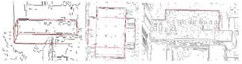
Figure 6. The extracted edge pixels and the final projection of the line segments of buildings: B1, B2, and B3.
Table 3. The optimal exterior orientation parameters and the differences compared to aerial triangulation.
| Exterior Orientation Parameters | 3 Building Models (26 Control Line Segments) | 5 Building Models (45 Control Line Segments) | ||||
| LSMIF | Aerial Triangulation | Differences | LSMIF | Aerial Triangulation | Differences | |
| X0 (m) | 168847.437 | 168847.386 | 0.051 | 168842.978 | 168847.386 | -4.408 |
| Y0 (m) | 2544722.612 | 2544703.908 | 18.704 | 2544704.213 | 2544703.908 | 0.305 |
| Z0 (m) | 1609.918 | 1607.693 | 2.225 | 1606.999 | 1607.693 | -0.694 |
| (degree) | -1.222599 | -0.570264 | -0.652335 | -0.587379 | -0.570264 | -0.017115 |
| (degree) | -3.250736 | -3.279205 | 0.028469 | -3.430583 | -3.279205 | -0.151378 |
| (degree) | 86.325791 | 86.470850 | -0.145059 | 86.485610 | 86.470850 | 0.014760 |
5. Conclusion
A novel method for recovering image orientation by fitting 3D line segments to edge pixels has been developed and successfully tested for both close- range and aerial images. The advantage of the proposed method is that the edge pixels are extracted by automated algorithm and there is no need of manual measurement. The 3D line segments can be easily derived from existing maps or building models to provide higher-level constraint than traditional control points. Furthermore, the control line segment does not have to be entirely visible on the photo, the LSMIF is still able to solve orientation parameters and achieve satisfying accuracy even if some object occludes a part of the line. However, there is one requirement for the line segments that they should be evenly distributed in the i mage to ensure the geometric constraint. It is also important to carefully select a suitable buffer range for each projected line segment. The wide buffer might include irrelevant pixels and leads to incorrect fitting, yet narrow buffer could miss the real edge pixels and result in failure. Therefore, the buffer range should be variable depending on the accuracy of the approximate parameters and the extracting result of edge-detecting algorithm. Trying different edge- detecting algorithms to extract the most desirable edge pixels and the less irrelevant pixels will certainly improve the fitting results. Since there are usually plenty of redundant observations when using the proposed method, it is advised to remove the line segment that is close to many irrelevant or noise pixels from the LSMIF function.
6. Acknowledgments
This research is sponsored under the grants of projects NSC 90-2211-E- 006-103 and NSC 91- 2211- E-006- 092. The authors deeply appreciate for the support from the National Science Council of the Republic of China.
References
- Buchanan, T. , 1992. Critical Sets for 3D Reconstruction Using Lines. Computer Vision – ECCV, Berlin, Germany, pp.730-738.
- Chio, S., 2001. A Practical Strategy for Roof Patch Extraction from Urban Stereo Aerial Images , Ph.D. Dissertation of Department of Surveying Engineering, National Cheng Kung University, Taiwan, R.O.C.
- Ebner, H. and G. Strunz, 1988. Combined Point Determination Using Digital Terrain Models as Control Information, In: International Archives of Photogrammetry and Remote Sensing, Kyoto, Vol. XXVII, Part B11/3, pp.578-587.
- Forkert, G., 1996. Image Orientation Exclusively Based on Free-form Tie Curves. In: International Archives of Photogrammetry and Remote Sensing, Vienna, Vol. XXXI, pp.196-201.
- Förstner, W., 1994. A Framework for Low Level Feature Extraction, Computer Vision, Springer- Verlag, pp. 383-394.
- Fuchs, C., 1995. Feature Extraction, Second Course in Digital Photogrammetry, IFP University Bonn, pp. p.3-1~p.3-36.
- Fuchs, C. and W. Förstner, 1995. Polymorphic Grouping for Image Segmentation, The 5th ICCV'95, Boston, pp. 175-182.
- Haralick, R. M. and Y. H. Cho, 1984. Solving Camera Parameters from The Perspective Projection of a Parameterized Curve. Pattern Recognition, 17(6), pp.637-645.
- Jaw, J. J., 1999. Simultaneous Determination of Exterior Orientation and Terrain Surface from Aerial Imagery and Scanning Airborne Laser. In: International Archives of Photogrammetry and Remote Sensing Commission III Symposium, Columbus, Ohio, USA, pp.52-57.
- Liu, Y., Huang T., and O. Faugeras, 1990. Determination of Camera Locations from 2D to 3D Line and Point Correspondences. IEEE Transactions on Pattern Analysis and Machine Intelligence, 12(1), pp.28-37.
- Mulawa, D. C. and E. D. Mikhail, 1988. Photogrammetric Treatment of Line ar Features. In: International Archives of Photogrammetry and Remote Sensing, Washington D.C., Vol. XXIX, Part B3, pp.383- 393.
- Mulawa, D. C., 1989. Estimation and Photogrammetric Treatment of Linear Features. Lafayette, Ph.D. Thesis, Purdue University.
- Petsa, E. and P. Patias, 1994a. Sensor Attitude Determination Using Linear Features. In: International Archives of Photogrammetry and Remote Sensing, Como, Vol. XXX, Commission I, pp.62-70.
- Schenk, T., 1999. Digital Photogrammetry. Laurelville Ohio, TerraScience, pp.399-415.
- Schwermann, R., 1994. Automatic Image Orientation and Object Reconstruction Using Straight Lines in Close- range photogrammetry. In: International Archives of Photogrammetry and Remote Sensing, Melbourne, Vol. XXX, Commission V, pp.349-356.
- Smith, M. and D. Park, 2000. Absolute and Exterior Orientation Using Linear Features. In: International Archives of Photogrammetry and Remote Sensing, Amsterdam, Vol. XXXIII, Part B3, pp.850-857.
- Zalmanson, G., 2000. Hierarchical Recovery of Exterior Orientation from Parametric and Natural 3-D Curves. In: International Archives of Photogrammetry and Remote Sensing , Vol. XXXIII, Part B2, pp.610- 617.
- Zielinski, H., 1992. Line Photogrammetry with Multiple Images, In: International Archives of Photogrammetry and Remote Sensing, Washington D.C., Vol. XXIX, Part B3, pp.669-676.