GISdevelopment.net ---> AARS ---> ACRS 2002 ---> Hyperspectral Data Acquisition and System Data Exploration and Analysis of Hyperspectral images: Visualization and Symbolic Description Pai-Hui Hsu PhD Candidate Department of Surveying Engineering National Cheng Kung University Yi-Hsing Tseng Associate Professor No.1, University Road, Tainan 701, TAIWAN Tel: +886-6-2370876 Fax: +886-6-2375764 Email: p6885101@ccmail.ncku.edu.tw Republic of China Abstract: Some visualization techniques are used to analyzing and exploring the data set of hyperspectral images. The major objectives of data analysis are to summarize and interpret a data set, describing the contents and exposing important features. For dimensionality reduction, visualization can play an important role in illustrating the characteristics of high dimensional data set. Data projection is one of the common visual ways to get the interesting subsets of the original data, and certain properties of the structures can be preserved as faithfully as possible. The difference between different classes can also be interpreted by projecting the class data to special data spaces. Some characteristics and inherent properties of hyperspectral images will emerge from the visualizations for dimension reduction and classifications. 1. Introduction Imaging spectrometers have been developed to acquire hyperspectral images with several hundreds of spectral bands. For example, the AVIRIS scanners developed by JPL of NASA can provide 224 contiguous spectral channels. Providing such abundant spectral data should increase the abilities in classifying land use/cover types. However, due to the high dimensionality and high correlation between spectral bands, traditional classification approaches do not fit to classify the hyperspectral images. To overcome the problems, one promising approach frequently used by many hyperspectral processing systems is dimensionality reduction. The basic principle of dimensionality reduction should extract the significant features or structures, and eliminate the redundant information. These useful features or structures can take the form of trends, clusters, hypersurfaces, or anomalies and can be used for further applications such as data compression or classifications. In order to perform the dimensionality reduction effectively, the analyst should fully understand the characteristics of hyperspectral data. Some characteristics of high dimensional space were studied for feature extraction of hyperspectral images (Jimenez and Landgrebe, 1998). One of the apparent characteristic is that high dimensional space is mostly empty. For examples, the volume of a n-dimensional hypercube with edges of length 2r is (2r)n. 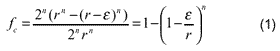The fraction of this volume that is contained between the surface and a smaller hypercube with edges of length 2(r-e) is Note that lim n®¥ fc =1,"e > 0, implying that most of the volume of a hypercube is concentrated in an outside surface. In other words, in a high-dimensional hypercube region, most of the available space is spread around the surface of the region. The same is true of regions with other hyper-shapes, such as the hypersphere and hyperellipsoid. This property prompts us to reduce the dimensionality of hyperspectral images by projecting the data to a smaller dimensional subspace without losing significant information. The remainder problems are what the clear definition of features is and how to design the algorithms of feature extraction. In order to give a definition of features which are helpful for dimensionality reduction, it is necessary to explore the data set via the visualization or symbolic representation. The major objectives of data analysis are to summarize and interpret a data set, describing the contents and exposing important features. Visualization can play an important role in data exploring and analysis. For example, the image cube is often used to represent the whole data set of the hyperspectral images. Several graphical methods have been proposed for visualizing high-dimensional data items directly, by mapping the apparent data values of each dimension into one figure. Data projection is the common visual way to get the interesting subsets of the original data, and certain properties of the structure of the data sets can be preserved as faithfully as possible. In this paper, some projection methods are used to explore and analyze the hyperspectral images. In addition, the multi-scale approaches are used to visualize the hyperspectral curve in a time-scale plane. The useful features then can be explored and extracted for further applications. An AVIRIS data set with five classes is used to demonstrate the ways of visualization and symbolic description. 2. Visualization Techniques For the convenience of analyzing and quantifying the characteristics of hyperspectral data, it is necessary to define mathematically and conceptually some representation spaces to inspect the data variations from some aspects. Landgrebe (1997) illustrated that there have been three principle ways in which multispectral data are represented quantitatively and visualized. Figure 1 shows three different data spaces which are used to represent multispectral images. The same representations are still convenient for hyperspectral data. In this paper, some extended methods of the three visualization techniques are described to characterize the hyperspectral images. 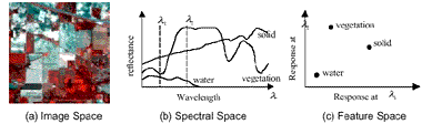Figure 1. Three data space for representing multispectral data 2.1 Spatial-Spectral Space Data in the RGB image space (see figure 1.a) directly offer a visual way to understand the spatial variation of the scene and the relationship between an individual pixel and the land cover class it belongs to. Tasks of manual image interpretation are usually carried out in the image space. However, the RGB image only shows the spatial information of three bands corresponding to Red, Green and Blue. In contrast to RGB images, the spectral slices are used to extract a combined spatial/spectral profile from a hyperspectral image. Figure 2.a shows a spectral slice with two classes. The vertical direction corresponds to the spatial dimension of the image being slices, the horizontal direction corresponds to the spectral dimension, and the grayscale shows the spectral density (reflectance, radiance, etc.). By a perspective view, a which creates a RGB image with the spectral slice of the top row and right column can be displayed on the 2D screen. Figure 2.b shows a hyperspectral image cube. 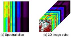Figure 2. 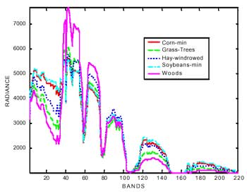Spatial-spectral space 2.2 Spectral Space The spectral response of a material can be defined as a spectral signature by the reflectance or radiance as a function of wavelength. Therefore, the spectral variations of each pixel can be drawn as a curve on the spectral space (see figure 1.b). Theoretically each class related to the composition of different material has its own shape and variance of the spectral curve. Some methods like “spectral matching” and “spectral angle mapper” use this property to distinguish the unknown spectral curve comparing with a series of pre-labeled spectral curve. Figure 3 shows the spectral signature of five different classes. Some basic statistics are calculated to depict the characteristics of the spectral variation. The mean curve represents the trend of the spectral variation. The standard deviations show the scattering to the mean. The maximum and the minimum values present the range of variation. One may find that the Grass-Trees and Hay-windrowed have very similar mean spectral curve, but present very different stadard deviation, maximum and minimum values. Different spectral curves can be portrayed on one spectral space for comparison. Figure 4.a shows the overlaps of five different spectral signatures. The spectra can also be offset vertically to allow interpretation (see figure 4b). 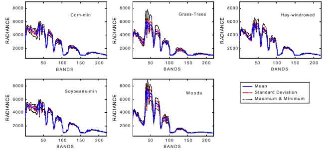Figure 3. The spectral signature of five different materials. 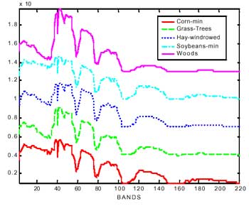(a) Overlap spectral data (b) Stack spectral data Figure 4. Different spectral curves in the spectral space. 2.3 ScatterPlots Scatterplots are one of the oldest and most commonly used methods to project high dimensional data to a 2D space. In this method, n*(n-1)/2 pair-wise parallel projections are generated, where n is the number of dimensionality. Each scatter plot gives the analyst a general impression regarding relationships within the data between pairs of dimensions. Figure 5.a show a 2D scatter plot of fi ve different classes with band 24 and 37. The pixels within one class cluster together and can be considered as a pattern. Thus the characteristics of classes can be interpreted by “pattern recognition” based on the statistic approach (Swain and Davis, 1978). For example, the separability analysis calculates the distances between two different classes for various band combinations. Then the bands with large distance can be selected as useful features. Scatter plot can be extended to 3D space. Figure 5.b. shows the 3D scatter plot with band 24, band 31 and band 37. The 3D scatterplot can be rotated interactively by users to an appropriate view point. Figure 5.c shows the Mahalanobis distance of each class pair. One may notice that the Mahalanobis values are corresponding to the geometric Euclidean distance between different classes on the 2D and 3D scatterplot. 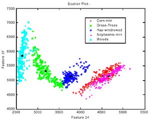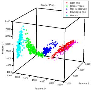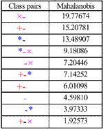(a) 2D scatter plot (b) 3D scatter plot (c) The Mahalanobis distance of each class pair Figure 5. 2D and 3D scatterplots and the Mahalanobis distance between two classes. 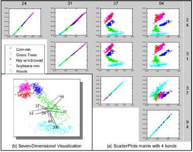Figure 6. Scatterplot matrix and m-dimensional visualization. Scatterplot matrix can be used to represent several scatterplots simultaneously to see the relationships between 3 or more bands. Figure 6.a shows a scatterplot matrix with band 24, 31, 37 and 94. The dialog of scatterplot matrix shows the high correlation of one band. Figure 6.b shows that the correlation between bands 24 and band 31 is very high, and the Grass-Tree between bands 24-37 and bands 31-37 have opposite correlations. When the number of bands is larger than 3, spectra can also be thought of as points in an m-dimensional scatterplot, where m is the number of bands (Boardman, 1993). The coordinates of the points in m-space consist of “m” values that are simply the spectral radiance or reflectance values in each band for a given pixel. The distribution of these points in m-space can be used to estimate the number of spectral endmembers and their pure spectral signatures (Boardman et al., 1995). Figure 6.b shows the 7-dimensional Visualization of Hypersepctral data which is created by ENVI’s n-Dimensional Visualizer TM . The user can interactively select the endmembers in m-space. 2.4 Statistics Images The importance of the second order statistic in discriminating between classes in high dimensional space was illustrated by Lee and Landgrebe (1993). As the dimensionality increases, the class covariance differences become more important, especially when adjacent bands are highly correlated. An effective visualization tool for second-order statistics is the statistics image. The class covariance or correlation matrix is displayed as a pseudo colored maps, the color indicate the degree of covariance between bands, from negative to positive values. Figure 7 shows the statistic images of covariance matrix (the upper row) and correlation matrix (the lower row) corresponding to five different classes. The correlation matrices show that the absorption bands will have low correlation coefficients. As a glance, one can subjectively perceive how each band is correlated and easily compare the statistics of the different classes. 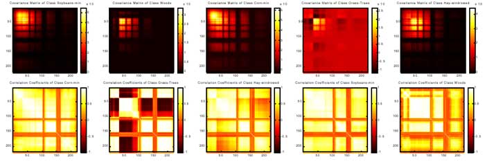Figure 7. Statistic Images of five classes. 3. Symbolic Representation A symbolic description called finger-prints of the absorption bands for hyperspectral data was developed by Piech and Piech (1987, 1989). The finger-print is a representation based on a scale space filtering of the hyperspectral data. A scale space image is a set of progressively smoothed versions of the original spectral curve. As the smoothing scale increase, features of the curve disappear until only a dominant spectral shape remains. The net result of scale space analysis of a hyperspectral data curve is a sequence of triplets. Each triplet describes a spectral feature and contains a measure of important directly related to the area contained within the spectral feature and the left and right inflection points of the spectral feature. Another method to produce similar finger-prints using wavelet transform was proposed by Hsu (2000). The wavelet transform can focus on localized signal structures with a zooming procedure. By detecting the positions of zero-crossing and modulus maxima of wavelet coefficients, the fringe-prints can be delineated and will correspond to the positions of absorption bands. The positions of zero-cross represent the variations of a spectral curve, and the positions of modulus maxima point out the inflection points Besides, the method proposed by Hsu is helpful for spectral analysis to reduce the dimensionality of hyperspectral data. Finally, a smaller number of key features can be both automatically processed and physically interpreted. Figure 7.a shows the wavelet coefficients represented by a pseudo colored map. Figure 7.b shows the zero-crossing of wavelet coefficients which are calculated by the wavelet function of first derivative of Gaussian, Sombrero and Morlet respectively. The modulus maxima of the coefficients calculated by Gaussian, first derivative of Gaussian Sombrero and Morlet functions are shown in figure 7.c. Figure. 8 The finger-prints of a spectral curve using wavelet transform 3. Conclusions The high spectral resolution characteristic of hyperspectral sensors preserves important aspects of the spectrum and makes differentiation of different materials on the ground possible. However, due to the high dimensionality and high correlation between spectral bands, traditional analysis approaches do not applicable to process the hyperspectral images. It is necessary to reduce the dimensionality before the processing of hyperspectral data. The main objective of data analysis is to summarize and interpret a data set, describing the contents and exposing important features. Visualization can play an important role in data exploring and analysis. In this paper, some projection methods are used to explore and analyze the hyperspectral images. The features can be selected from the scatterplots and the endmembers can be obtained from the n-dimensional visualization. In addition, the multi-scale approaches, such as the finger-prints and wavelet transform are used to visualize the hyperspectral curve in a time-scale plane. The useful features then can be explored and extracted for further applications. Acknowledgment The authors would like to thank the National Science Council of Republic of China, for support of this research project: NSC89-2211-E006-118. References Boardman, J. W., 1993. Automated Spectral Unmixing of ARIRIS data using convex geometry concepts: in Summaries, Forth JPL Airborne Geoscience Workshop, JPL Publication 93-26, Vol. 1, pp. 11-14. Boardman, J. W., Kruse, F. A., and Green, R. O., 1995, Mapping target signatures via partial unmixing of AVIRIS data: in Summaries, Fifth JPL Airborne Earth Science Workshop, JPL Publication 95-1, Vol. 1, pp. 23-26. Hsu, P.-H. and Tseng, Y.-H, 2000. Wavelet-based Analysis of Hyperspectral Data for Detecting Spectral Features, XIXth Congress of The International Society for Photogrammetry and Remote Sensing (ISPRS). July 16-23, 2000. Amsterdam, Netherlands. TP VII-10-17 / 602. Jimenez, L. O. and Landgrebe D. A., 1998. Supervised Classification in High-Dimensional Space: Geometrical, Statistical, and Asymptotical Properties of Multivariate Data. IEEE Transactions on Geoscience and Remote Sensing, 28 (1), pp. 39-54. Landgrebe, D.A., 1997. On Information Extraction Principles for Hyperspectral Data (A White Paper), obtained from http://dynamo.ecn.purdue.edu/~biehl%20/MultiSpec/documentation.html. Lee, C. and Landgrebe D. A., 1993. Analyzing High-Dimensional Multispectral Data, IEEE Transactions on Geoscience and Remote Sensing, 31(4), pp. 792-800. Piech, M. A. and Kenneth, R. P., 1987. Symbolic representation of hyperspectral data, Applied Optic, 26(18), pp. 4018-4026. Piech, M. A. and Kenneth, R. P., 1989. Hyperspectral interactions: invariance and scaling, Applied Optic, 28(3), pp.481-489.