| GISdevelopment.net ---> AARS ---> ACRS 2002 ---> Earth Observation from Space |
Landsat ETM+, Terra MODIS and
NOAA AVHRR: Issues of scale and inter-dependency regarding land
parameters
Thomas Alexandridis
Ph.D. student in remote sensing and GIS applications (Aristotle Univ. of Thessaloniki)
13 Milona Street, Thessaloniki 54636, Greece
Tel: (30)- 310 -998778
E-mail: thalex@agro.auth.gr
Greece
Yann Chemin
PhD student in remote sensing applications (AIT-STAR)
206/7 Kamathawatte Road, Rajagiriya, Sri Lanka
Tel: (94)- 1-886053
E-mail: ychemin@yahoo.com
France
Abstract
Space observation has enjoyed increasing interest from various sides of resources management over the last decades. Within the past few years, the cost of data acquisition and processing has dropped, and a large amount of satellite data is already available on the Internet, free of any charge. This plethora of data has the advantage of bringing directly usable information to a wider range of users, both to scientists and to a larger, less specialized public. Whatever the case, the initial choice of the dataset depends on various parameters and special attention should be given to this. Under these conditions and with such an ungrudging supply of satellite data, the question arises: which is ‘better’ for a given application? But also, what does ‘better’ mean?
In this paper, three sensors used for the monitoring of vegetation are evaluated: NOAA AVHRR, Terra MODIS and Landsat ETM+. Although the issues of scale are the primary focus, the differences in calculating land parameters using imagery from these sensors are attributed to spectral, technical and scale factors. Multi-resolution analysis is performed on the examined datasets in order to identify the optimum scale of observation of vegetation in the study area. Moreover, the possibility of substitution of one with another is evaluated through checking the correlation coefficients between the datasets. Although it is believed that higher spatial resolution gives more accurate results in measurements made with remote sensing data, there is an indication that highest variability is explained by the vegetation index image of MODIS sensor, which leads to the conclusion that this may be the optimum sensor for this application. The level of similarity of the vegetation index pattern calculated from the three sensors is not uniform, indicating that different sensors depict different characteristics of the ground. Valuable comments are made in the discussion regarding the usefulness of moderate resolution satellites.
1. Introduction
Remote sensing of land parameters has gained a lot in recognition since the high spatial resolution satellites for monitoring vegetation were launched in the late 70s. Since that time, research evolved in the applications of remote sensing for land management, towards developing methods to use satellites of various spatial resolution in monitoring of environment. Often reserved to scientists, because of cost and heavy calibration physics and processing, satellite imagery has become recently more affordable (in some cases even free). More important, a large amount of data preparation is now commonly performed before delivery. This makes satellite information more accessible to users, that require now only knowledge at the application level.
Available from the end of 1988, the 1.1 Km spatial resolution NOAA AVHRR satellite is the combined land and climate purpose sensor that is now the most widely used in medium to large area investigation. Its high spatial resolution correspondent is the Landsat series. Launched in 1999, Landsat 7 ETM+ is having 15- 30m visible and 60m thermal sensing pixel size. Earlier Landsat missions are not providing the comparative pre-processing level of NOAA AVHRR and Landsat 7 ETM+, making the transfer of its use to end-users a complex task. More recently (2000), MODIS sensor (on -board of Terra satellite) is roviding information from 250m to 1Km spatial level. Attractive advantage of MODIS is that a large amount of effort has been put into the development of directly usable pro ducts (information) after the processing of the data from the MODIS Science Team.
The first hindrance found in having high spatial resolution satellite images like Landsat is that information is not available very often (i.e. 16 days) while satellite of bigger pixel sizes are revisiting the same part of the earth very often. To overcome this, the technique of combining data from more than one satellite, to take advantage of high temporal and high spatial resolution, is commonly used. Moreover, a difference in the output signal of the three sensors is expected since each sensor is capturing the reflected energy in varying band widths. In Table 1 are listed the band widths of the red and near-infrared bands of the three sensors and their radiometric resolution. Both ETM+ and MODIS red and near-infrared spectral bands are narrower than those of AVHRR, causing different response from vegetation, which in turn alters the computed vegetation index. The narrower width in the near-infrared part of the spectrum elimi nates the effect of the water absorption region (around 950 nm and 1100 nm), and also renders the red band more sensitive to chlorophyll absorption (van Leeuwen et al., 1999). However small these effects, can give significant differences in vegetation response of dense canopies and multiple leaf layers (Hoffer, 1978).
Table 1: Band widths and radiometric resolution of red and near-infrared bands.
|
| |||
| sensor | red (nm) | near-infrared (nm) | radiometric resolution |
|
| |||
| ETM+ | 630-690 | 750 -900 | 0-255 |
| MODIS | 620-670 | 841 -876 | 0-4095 |
| AVHRR | 580-680 | 725 -1100 | 0-1023 |
|
| |||
Vegetation indices have become a common tool in monitoring vegetation change, for land cover classification, for calculation of leaf area index and biomass production. They provide a spatially distributed indication of chlorophyll appearance, easily calculated from satellite spectral bands, which is their main advantage.
Primary objective of this paper is to assess the differences of land parameters calculated through various sensors. A key land parameter under consideration is the vegetation index NDVI, and the examined sensors are two widely used and a recently available one. Another objective is to attribute the differences to spectral, technical and scale factors, and check the possibility of substitution of one with another.
1.1 Study Area
Situated in the Hubei Province, Central China, the Zhanghe Irrigation District is a sub-basin north of the Yangtze Changjiang River. The net irrigated area reported is approximately of 160,000 ha, providing a large proportion of Hubei Province grain production. Rice production is widespread in the irrigation system, and the recent decline in water availability to agricultural purposes has not decrease much the global rice production due to a proportional increase of efficiency of water use by the farmers (Dong et al., 2001). The undulating terrain is constraining the size and shape of the fields, and their discrimination is a difficult task, even with higher resolution satellites.
2. Data and Processing
A MODIS satellite image was acquired on the July 10, 2000, approximately 15 -25 minutes after the acquisition of the Landsat ETM+ image. There are numerous little clouds covering the Zhanghe Irrigation District, but not exceeding 8 percent of the area. The haze which is observed in the north east and south part of the ETM+ image is not so evident in the MODIS image, probably due to the later time of overpass, or due to spectral differences. The NOAA AVHRR image used in this study is captured on July 9, 2000, since there were no images available in the Satellite Active Archive for July 10. It is a cloud free image, and possibly existing small clouds are not visible due to low resolution.
Except from the original band data, vegetation index products can also be ordered from the EOSDIS center. These are 16 days maximum NDVI (normalized difference vegetation index) and EVI (enhanced vegetation index), aggregated in 500 m pixel size, with a product name MOD13A1. A compositing algorithm is implemented from the MODIS Science Team to account for cloud cover in the 16 days period that each product covers (van Leeuwen et al., 1999). Two sets of products have been used, one covering maximum NDVI from June 25 to July 10, 2000 (MOD16a), and the other from July 18 to July 26, 2000 (MOD16b). Alth ough there are no missing data, the effect of partial cloud cover is evident in the data set MOD16a.
The spectral bands of Landsat 7 ETM+ were checked upon atmospheric disturbance by creating the broadband surface albedo (Equation 1) after the method found in Ahern et al. (1977) and Koepke et al. (1985). It was validated against the physical features value of albedo (Table 2) taken from Tasumi et al. (2000).
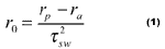
where r0 is the broadband surface albedo (-), rp the planetary reflectance (-),ra the in-band path solar irradiance (-) and tsw the single-way transmittance of the atmospheric layer (-).
Table 2: Expected broadband surface albedo after Tasumi et al. (2000)
|
| |||
| Physical Feature | Expected Albedo | Broadband | Surface |
|
| |||
| Grass or Pasture fields | 0.15 to 0.25 | ||
| 0.14 to 0.22 | |||
| Paddy Field (Rice) | 0.17 to 0.22 | ||
| Water (30° < solar elevation < 50°) | 0.025 to 0.06 | ||
|
| |||
Mainly the Northern part of the Zhanghe Irrigation District was affected by what was presupposed to be morning haze. The reflectance values were found to be very close to the expected values in most of the other parts of the image, and therefore it was expected that NDVI calculation would give correct results. Expected deviation of NDVI was located only in the most northern part of the study area for reasons stated above. Because of the very good band- wise reflectance from Landsat that do not require atmospheric corrections, it was proposed to calibrate the MODIS and AVHRR bands to the Landsat ones. Two areas with extreme reflectance values where selected, the maximum one being situated at the most northeastern part of the Zhanghe Irrigation District, being irrigated cotton crop. The minimum val ue sample site was selected as being the Changjiang reservoir, downstream and in the southeastern of the study area. Correction levels to band -wise reflectance were applied consequently to the MODIS and AVHRR image assuming the Landsat image as reference. NDVI was subsequently extracted from the images from the newly calculated surface reflectance in Band 1 and 2.
2.1 Multi-Resolution Analysis
The exploration of scaling in remote sensing is sometimes based on multiple levels of observations (satellite images), but usually depends upon the analysis of original data at multiple resolutions created by some kind of generalization operator g( ) that should not introduce artifacts into the data (De Cola, 1997). In this study, satellite remote sensing observations were acquired at three levels of scale, 30m, 250m and 1.1 km. The in between scale levels were simulated by aggregating the data with the average method (Bian, 1997). The grid layers created with this technique are called pyramid layers. Let level 0 be the scale of Landsat ETM+ image, which is based on a 30 m pixel size. The same scale level is inherited to the NDVI image produced, as described in a previous chapter. From this NDVI image, scale levels up to 1 km were simulated (Table 3). In a similar way, pyramid layers were created from the NDVI calculated from the original MODIS data, from scale level 3 (250m) to scale level 5 (1 km). Scaling down was carried out only up to level 5 and thus no multi -resolution analysis was conducted in the AVHRR image. A selected list of the pyramid layers produced is presented in Figure 1.
Table 3: Pyramid layers at various scale levels.
|
| |||
| Scale Level | |||
| Pixel size | ETM+ | MODIS | AVHRR |
|
| |||
| 30 m | 0 | ||
| 60 m | 1 | ||
| 120 m | 2 | ||
| 250 m | 3 3 | ||
| 500 m | 4 4 | ||
| 1 km | 5 5 5 | ||
|
| |||
3. Results
3.1 Optimum Scale
The optimum scale of observation is closely related to the operational scale, and is a function of the type of environment studied and the kind of information desired. In this study, when using NDVI images to describe vegetation, as optimum scale of observation can be defined the scale where the desired features are adequately depicted, avoiding excess of data. In literature it is defined as the scale where the “action” occurs, that is where the highest variability is described (Cao and Lam, 1997, Woodcock and Strahler, 1987). An example follows: if the spatial resolution is considerably finer than the features of interest on the ground, most of the pixels in the NDVI image would be highly correlated with their neighbors, and the local variance would be low. Equally low would be the local variance in case the resolution becomes much coarser, and many features are found in a single pixel. If the features of interest approximate the size of pixels, then the possibility for neighbors to be similar decreases and the local variance rises. Therefore, the optimum scale of observation can be identified by measuring the amount of variance in a NDVI image (De Cola, 1997), or the local variance (Woodcock and Strahler, 1987).

Figure 1: Selected images from NDVI pyramid layers.
Descriptive statistics were calculated from the NDVI images. The mean NDVI for the whole of Zhanghe Irrigation District calculated from various sources is shown in Table 4. The differences are negligible and probably due to spectral discordance, as discussed in the introduction. The drop in the variance is expected, when moving from high resolution data sets to low resolution. Nevertheless, MODIS shows the highest variance, which is indicating the sensor and scale where the highest variability is occurring, therefore identifying the optimum scale of observation.
Table 4: Descriptive statistics of the NDVI data sets.
|
| ||
| Sensor | Mean NDVI | Variance |
| ETM+ | 0.545 | 0.0151 |
| MODIS | 0.542 | 0.0169 |
| NOAA | 0.517 | 0.0049 |
|
| ||
| MOD16a Jun25-Jul10 | 0.494 | 0.0142 |
| MOD16b Jul18- Jul26 | 0.722 | 0.0052 |
|
| ||
Following the same trend, the global variance of the NDVI at various scale levels is dropping with the pixel size increasing (Figure 2a). This an inherent characteristic of grid data, which reveals the relation of pixel size with the ability to describe detailed features on the ground. The highest global variance is observed at MODIS scale level 3 (original) data set. From these sets of results, it can be concluded that the optimum scale of observation for vegetation in Zhanghe Irrigation District is level 3 with MODIS sensor.
3.2 Influence of Scale Change
Texture analysis has been proposed by various researchers (Cao and Lam, 1997, Woodcock and Strahler, 1987) as one of the techniques to examine the influence of scale and resolution change. With this technique, a 3x3 moving window is passing through the entire image, and the local variance is calculated in this window. Local variance is a method to examine the local particularities of the study area, that is the variation from the neighboring pixels. The average local variance of NDVI is calculated for various sensors at different scale levels and is presented in Figure 2b.
It can be seen from Figure 2b that in the scale levels examined, there is a trend of ETM+ local variance to drop with increase of pixel size, while the local variance from MODIS is increasing. This shows that different sensors can have dissimilar response to mul ti-resolution analysis, although the scenes are acquired almost at the same time and are having similar atmospheric characteristics. Evidently, the MODIS sensor is highlighting texture originating from objects approximately at the size of 500 m or 1 km, which are more evident in the MODIS bands rather than the ETM+. Such objects are possibly the large reservoirs of Zhanghe, or the Yangtze river. Local variance from NOAA is in a much lower level, since the original resolution of NDVI at 1.1 km is inadequate to describe the cropping patterns and characteristics of vegetation in the area.

Figure 2: Global and local variance at various scale levels.
3.3 Similarity Across Sensors
Calculation of correlation coefficients between grids is a method of testing the similarity and the level of substitution of one with another (De Cola, 1997). Since the comparison is based on pixel-by-pixel level, aggregation to the same pixel size is required. Therefore, only the following combinations were examined (Table 5). The association of NDVI calculated from ETM+ and MODIS is quite strong at scale level 3 (r = 0.744), and is increasing to r = 0.821 with the pixel size increasing (scale level 5). The effect of overestimating the correlation when moving to coarser resolutions is common among auto- correlated data sets. Moreover, the effect of a potential mis-registration between the images is weakening when aggregating neighboring pixels with averaging.
The correlation of AVHRR calcul ated NDVI with the other two NDVI data sets is quite low, although the overall NDVI mean is similar (Table 4), revealing differences in the spatial distribution of vegetation pattern, as recorded by the AVHRR sensor. Except from the different spectral char acteristics of AVHRR sensor, another source of dissimilarity may be the existence of little clouds on July 9, small enough not be detected with the 1.1 km resolution, but significantly influencing the spatial distribution of NDVI. Another possible reason for atmospheric dissimilarities, except from the different date, can also be the different time of satellite overpass, being afternoon for NOAA and morning for Landsat and Terra. Varying sun angle, view angle at a hilly terrain can give dissimilar results, which could be only corrected using bidirectional reflectance distribution function (BRDF) models.
Table 5: Correlation coefficients of NDVI and NDVI products at various scale levels.
|
| |||||||||||||||||||||||||||||||||||||||||||||||||||
The correlation coefficients between various MODIS products describing NDVI are also calculated (Table 5), after aggregating the single date MODIS NDVI to scale level 4 (500 m), to match the 16 day data. The level of correlation is generally high within these data sets. The lower association of NDVI of July 10 with the 16 day product that is covering the same period is probably because of cloud cover influence, that can be clearly identified in the 16 day product. Despite the difference in the mean NDVI values (0.542 to 0.722), there is a higher correlation of the single day NDVI of July 10 with the 16 day product of the later period of July 18 to July 26. This can be explained because of the higher similarity in the spatial pattern of vegetation, as there is less cloud interference in the two data sets.
4. Conclusions
Although believed that higher spatial resolution gives better results in measurements made with remote sensing data, the optimum scale for the observation of vegetation in Zhanghe Irrigation District is shown to be scale level 3 (pixel size 250m), and the higher variability is described by the MODIS sensor. This is possibly because the detailed spatial pattern of the small fields and other mixed land use components of the Zhanghe Irrigation District cannot be depicted by the ETM+ sensor, and the more evident pattern of the lowland irrigated patches can better be described by the MODIS sensor.
Land parameters calculated from MODIS and ETM+ sensors show significant similarity. Despite the fact that AVHRR and MODIS have a smaller factor of scale difference, their correlation is much lower. The fact that the AVHRR image is acquired a day later is not a reason for a significant change in the spatial pattern of vegetation. A change in the atmospheric conditions is more probable from one day to another, and the appearance of small clouds, which are not evident in low spatial resolutions. Other possible reasons are the spectral and technical dissimilarities, as well as the difference in the time of image acquisition.
The large objects appearing in the scene (Yangtze river, the Changjiang city and the Zhanghe reservoir) are not described with the same strength of spatial texture in the ETM+ and MODIS images at the same scale level. This inconsistent behaviour of the texture analysis at scale level 4 and scale level 5 reveals that different spatial patterns are depicted in different sensors, according to the scale level that each sensor is designed to operate at.
The MOD13A1 product can be compared with NDVI from single day MOD IS image, despite the visual differences. The differences are attributed to the frequent cloud cover of the season that the compositing algorithm cannot account for. Possible reason is the varying view angle of the scenes that composite the 16 day NDVI. Wi th varying view angles the spatial resolution varies, and renders image to image registration a difficult task. Moreover, the values of vegetation indices can be influenced at large off-nadir angles and large solar zenith angles. Undoubtedly, the compositing algorithm does not perform to the best during the monsoon season in Zhanghe Irrigation District.
References
- Ahern, F.J., D.G. Goodenough, S.C. Jain, V.R. Rao and G. Rochon. 1977. Use of clear lakes as standard reflectors for atmospheric measurements, in Proc. 11th Int. Symp. On Rem. Sens. of the Envir.: 731-755.
- Bian, L. 1997. Multiscale nature of spatial data in scaling up environmental methods. Scale in remote sensing and GIS, eds. Quattrochi, D.A and Goodchild, M.F., CRC Press, Inc., pp. 13-26.
- Cao, C. and N.S. Lam. 1997. Understanding the scale and resolution effects in remote sensing. Scale in remote sensing and GIS. eds. Quattrochi, D.A and Goodchild, M.F., CRC Press, Inc., pp. 57 -72.
- De Cola, L. 1997. Multiresolution covariation among Landsat and AVHHR vegetation indices. Scale in remote sensing and GIS. eds. Quattrochi, D.A. and Goodchild, M.F., CRC Press, Inc., pp. 73-92.
- Dong; B., R. Loeve, Y.H. Li, C.D. Chen, L. Deng and D. Molden. 2001. Water productivity in Zhanghe Irrigation System: Issues of scale. In: Barker, R.; Loeve, R., Li, Y. H., Tuong, T.P. (eds.). Water -saving irrigation for rice: Proceedings of an International Workshop held in Wuhan, China, 23- 25 March. pp. 97-115.
- Hoffer, R.M. 1978. Biological and physical considerations in applying computer-aided analysis techniques to remote sensor data. In: Remote sensing: The quantitative approach. eds. Swain, P. H., and Davis S.M. McGraw- Hill Inc., pp. 227-289.
- Koepke, P., K.T. Kriebel and B. Dietrich. 1985. The effect of surface reflection and of atmospheric parameters on the shortwave radiation budget. Adv. Space Res. 5: 351-354.
- Tasumi, M., W.G.M. Bastiannssen and R.G. Allen. 2000. Application of the SEBAL methodology for estimating consumptive use of water and streamflow depletion in the Bear River Basin of Idaho through Remote Sensing. Final Report. The Raytheon Systems Company, EOSDIS Project.
- van Leeuwen, W.J.D, A.R. Huete and T.W. Laing. 1999. MODIS vegetation index compositing approach: a prototype with AVHRR data. Remote Sens. Environ. 69:264-280.
- Woodcock, C.E. and A.H. Strahler. 1987. The factor of scale in remote sensing. Remote Sensing of Environment, 21:311-332.