| GISdevelopment.net ---> AARS ---> ACRS 2002 ---> Data Processing, Algorithm and Modelling |
Collaborating Remote Sensing
with historical limnological data to map primary productivity at a
Eutrophic lake
Pranab J.
Baruah
Post-doctoral fellow, Yasuoka Laboratory
Institute of Industrial Science, University of Tokyo
4-6-1 Komaba, Meguro-ku, Tokyo, 153-8505
Tel: (81)-3-5452-6415
Fax: (81)-3-5452-6410
E-mail: pjbaruah@iis.u-tokyo.ac.jp
Japan
Masayuki Tamura
Deputy Director, Social and Environmental Systems Division
National Institute for Environmental Studies
16-2 Onogawa, 305 0053
Tel : (81)-298-502479
Fax: (81)-298-502572
E-mail: m-tamura@nies.go.jp
Japan
Yoshifumi Yasuoka
Professor, Institute of Industrial Science
University of Tokyo 4-6-1 Komaba
Meguro-ku, Tokyo, 153-8505
Tel: (81)-3-5452-6409
Fax: (81)-3-5452-6411
E-mail: yyasuoka@iis.u-tokyo.ac.jp
Japan
Abstract
Primary productivity is a complex process, especially in shallow eutrophic inland waters, where there is considerable upwelling and mixing of bottom sediments during winds and considerable anthropogenic effects from the land-mass surrounding it. For mapping primary productivity by remote sensing in eutrophic lake therefore often involves costly and laborious sampling of the same simultaneous to the satellite overpass. This follows relating the lake-surface productivity to satellite retrieved radiances to develop some empirical algorithm for subsequent mapping. In this paper, a novel approach is presented where a satisfactory model based on historic limnological data of four parameters is utilized to map primary productivity at the lake Kasumigaura, Japan. The selected key water quality parameters, namely chlorophyll-a, suspended sediment, secchi disk depth and water temperature, can essentially represent the primary productivity and can be estimated from remote sensing imagery. The developed models can be used for any date of the year to generate satisfactory primary productivity maps at the lake by feeding the water quality maps of selected parameters as inputs. As the input variables are fewer, separate models for each month of a year is necessary for better approximation of the complex process of primary productivity. For the month of January, a neural network is successfully used to develop the productivity model with a coefficient of correlation (R2) >0.7 in both training and validation. Finally, a productivity map of Kasumigaura for 19th January, 2001 is generated for demonstration.
Introduction
Inland water bodies constitute less that 1% of the total water volume of the world and provide us with the much needed drinking water and water for agriculture. Inland water quality is directly affected by the conditions of the surrounded land mass and vice versa. To this very reason and others, inland water environment is quite complex and dynamic in both spatial as well as temporal scale. . The productivity in these waters is thus a very complex process and measuring and estimating the same provides valuable insight to the present situation. Limnologists have been using quite a number of components to depict the inland water quality and for decades, they have been depending on point samplings to assess the water quality in these waters. Although traditional point samplings are accurate, they are time-consuming and, do not provide the necessary spatial overview required to understand the processes which often vary with wide range of spatial scales (Harris, 1986). With the advent of remote sensing, several semi-analytical models have been developed to estimate primary productivity in oceanic environments from remotely detected chlorophyll concentrations (and assumed chlorophyll profile across depth) or sun-stimulated chlorophyll fluorescence (Esais et al. 1997). However, these algorithms do not work well in inland waters due to their optical complexity by virtue of multi-componancy. Moreover, the modern aquatic sensors are of no use in these waters as they are of coarser spatial resolution. Mostly, empirical models relating remote sensing reflectance with surface productivity are developed for mapping primary productivity in inland waters. However, this process is often costly and laborious as sufficient data samplings concurrent to satellite overpass are necessary for satisfactory estimation of the same. Moreover, a model developed with this method is often weak in temporal scale and often can not at all be used to map the productivity at other dates.

In our research, therefore, we developed a methodology whereby the productivity model is based on already existing pool of data (or data at regular intervals) of some limnological variables which can be effectively estimated by remote sensing and which essentially can represent the very process of primary productivity. This way, remote sensing capabilities are integrated with historical pool of limnological data for meaningful productivity mapping . The inputs to the models are water quality maps of the variables under consideration for a certain day and output is the primary productivity map of the water body. To ensure better representation of the complex phenomenon of productivity, neural network has been used. The historical pool of limnological data used in this study is from samplings spanning several decades spread over the lake.
Study Site and Limnological Data
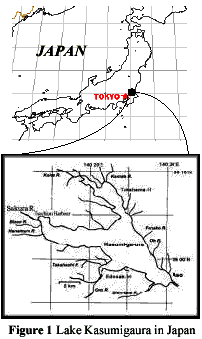
The study site is the lake Kasumigaura (fig. 1), the second largest lake with an estimated area of 220 km2 and with a total catchment area of 1969 km2. Originally a brackish type, it became a freshwater lake in 1976 after construction of a regulatory dyke at its only outlet preventing seawater from coming in. With an average depth of 4m and a maximum depth of 7m, it is an eutrophic lake throughout the year. The lake environment is crucial to the environment and the population of 950,000 residing around its banks in about 45 cities. Due to this very fact and the degrading water quality have attracted many national and international researchers to focus on analyzing the water quality problems and processes of lake Kasumigaura. Lake Kasumigaura Research Station of National Institute of Environmental Studies (NIES), Japan along with several other government as well as private organizations have been collecting data for supporting various researches on water quality of the lake to propose remedial measures for betterment of the solution. Lake Kasumigaura Databook (2001) published by Center for Global Environmental Research (CGER), NIES compiles limnological data for several important variables for 10 locations spread over the lake and taken at monthly intervals during the period 1977 ~ From the dataset, the mean chlorophyll concentration at Kasumigaura was 69þg/l (Max:199 ? g/l) in yr.2000 with a typical yearly sediment load of 67-91 t/ km2 from the 56 rivers feeding the same.
Aquatic Primary Production and Modeling Requirements
Aquatic primary production can be considered as the mass of carbon fixed as newly grown organic material in the water column. Thus it is the sum of all the photosynthetic rates within the aquatic ecosystem and often a synonym for aquatic biomass. Phytoplanktons provide the material basis for the pelagic ecosystem through primary production. However, excess primary production sometimes deteriorates water quality due to dense blooms of nuisance algae, causing serious damage to the fish production, recreation, flora and fauna as well as to the human health due to a variety of resultant substances such as CO2, H2S, CH4, corrosive gases, and toxins (Falconer, 1993). Lake Kasumigaura is facing similar problems, and thus it is necessary to understand the chemical, biological and hydrological bases of controls on primary productivity in order to accurately predict the effects of inputs (nutrients from catchment) and to develop management strategies that can protect ecosystem functioning.
Empirical modeling of phytoplankton primary production (PP) has always been based on predictive variables that are more easily available and cheaper to measure than primary production. These mathematic models involve aquatic optics and chlorophyll concentration to predict phytoplankton primary production by analytical means (Cole et al., 1987). However, the analytical methods, with many assumptions, often can’t represent the underlying complexity typical to primary production. Modeling primary production has been a challenge and there are limited publications on the same. Neural network has been found to be a better solution for tackling the inherent non-linearity with some degree of success (Scardi, 1996, 2000; Scardi et al., 2001). However, the context of ecological modeling is quite different from that of most neural network applications, as data sets and knowledge are often very limited with respect to the complexity of the real world processes. Therefore, relationships between variables are only partly known and understood as they are usually studied by analyzing correlations rather than by defining causal pathways in a strictly deterministic framework (Scardi et al., 2001). In our research also, we selected neural networks for developing the primary productivity model for lake Kasumigaura.
Methodology
- Selection of variables
The major factors determining aquatic primary production for any given day is the biomass of phytoplankton, which itself results from previous production. Photosynthetic variation occurs through attenuation of photosynthetically active radiation (PAR, 400 ~ 700nm). Therefore, incident solar radiation and underwater light attenuation are the fundamental factors controlling the productivi ty of shallow lakes. According to Takamura et al. (1991), primary production in lake Kasumigaura is closely related to water temperature, solar radiation and chlorophyll-a concentration. Nutrients are found not to be the limiting factors of productivity. Concluding from the above discussion and a preliminary regression analysis on various limnological parameters and productivity, four limnological variables, namely, chlorophyll-a (chl.a, þg/l), suspended sediment (SS, mg/l), secchi disk depth (SDD, cm) and water temperature (WT, °C) are selected as input variables. Suspended sediment and secchi disk depth are used to simulate the effects of underwater light intensity. Sediments in fact play a significant role in the process of lake eutrophication, especially the clay size fractions. The first three optically active variables and WT can be estimated from broad-band sensors such as LandsatETM+. Broad-band satellite sensors are preferred to modern aquatic satellite sensors (e.g. MODIS) in inland waters due to their better spatial resolution.
Gross productivity (gm.C.m-2 day -1 ) data for lake Kasumigaura is available monthly from 1977 to 1996 for 10 stations spread over the lake. However, data prior to 1981 were not considered in this study as productivity was measured using O2 method from 1977 ~ 1980. Use of 13 C has been used since then for the measurement as radioisotopes such as 14 C is legally limited in Japan.
- The Quickprop neural network
For modeling, a faster variation of back-propagation neural network, namely, Quickprop is used. Quickprop, developed by Fahlman (1988) is not an adaptive learning technique. However, like any other back-propagation neural network, the network contains three kinds of typical layers, namely, input, output and hidden layers. All layers have processing units called nodes. Number of input nodes and output nodes and fixed and are based on number of variables under consideration. Number of hidden layers and hidden layer nodes may vary depending on the complexity of the problem. All nodes are interconnected in a forwardly manner with weighted interconnection. Finding the right combination of weights in these interconnections, which represents the system under investigation, is the goal of the network training. For this purpose, first, inputs are fed through the input layer and after passing through a summation and squashing function, the output becomes the input for the subsequent layer. This process continues until the final output is available at the output layer. The difference between the final output and the targeted output is then back-propagated for updating the weights in the interconnection. The weight update rule in Quickprop differs from conventional back-propagation algorithm and is dominated by a quadratic term,

where, S(n)? ?E/?w(n) The numerator is the derivative of the error with respect to the weight and S(n?1)?S(n)/?w(n?1)/ (S(n is a finite difference approximation of the second derivative. Together these approximate Newton’s method for minimizing a one-dimensional function : f (x)/ ?x? ? f(x)/f(x). To avoid taking an infinite backward step, or a backward uphill step, a maximum growth factor parameter ? is introduced. No weight change is allowed to be larger than þ times the previous weight change. Quickprop has a fixed learning rate that needs to be chosen to suit the problem. Detail discussion on back-propagation neural network and Quickprop can be found in Fausset (1994) and Reed et al.(1998) respectively.
- Model development
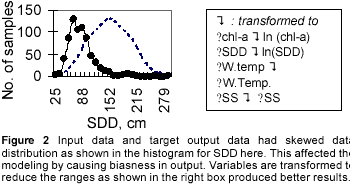
In our case, input variables are fixed at four selected variables. Output is the Gross Productivity (GP) at the lake. As a starting step, some trial training runs were made with the entire data set. It was found that, using all the samples from 1981 to 1996 could not produce a satisfactory model, as the input variables were limited. Even with a network with two hidden layers, it was difficult to train on the data set satisfactorily and a coefficient correlation (R2 ) above 0.5 could not be obtained. After examining and some trial and error on training on the data, it was found that, focusing the modeling on a certain season gave much better result than using the whole dataset. This is because productivity in lake itself being a complex process varies considerably with seasons in a typical year. Thus with fewer variables it becomes difficult to approximate a complex function. The situation is much more difficult when the approximating model is made independent of both the time and space component. Relaxing the model towards?the time-component can thus provide better results. It was found that, due to skewed data distribution (example shown in fig. 2) for the input variables, there was bias in the outcome of the network. Therefore, prior to training, variables were transformed to lower ranges by applying logarithm or square root, which produced better fit to both training and validation data. Thus, a moving-month model is proposed where a productivity model for each month of a year is proposed. To demonstrate the strategy, a model for the month of January is shown in detail with results. January was selected as water quality maps for the four input parameters were available for 19 th January, 2001 which were again generated from LandsatTM imagery on that day (Baruah, 2002). The strategy in the moving month model is to select data for two immediate neighboring months for modeling to the month for which the model is being developed. Thus, for the model of January, we extracted data for the three months, namely, December, January and February. A total of 80 samples were available for these three months. As the training samples were limited we used Quickprop with cross-validation by randomly selecting 90% of samples as training data and the rest as validation data, so as to avoid local minima while training. A single hidden layer is used. Number of hidden layer nodes was varied to arrive at the optimum number, which gave least overfitting and best weight configuration. A network trained with Quickprop and 5 hidden layer nodes (i.e. a 4-5-1 network) was found to give the best weight configuration with a weight growth rate of 1.75 at epochs (iterations) of 22256.

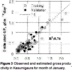
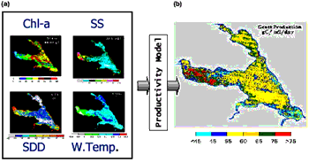
As seen from the graphical representation of the results (fig.3), the model could represent the winter productivity at lake Kasumigaura quite well from the input variables of chl-a, SS, SDD and WT satisfactorily. Composite coefficient of determination (R 2 ) taking into account both the training and validation dataset was 0.76. With satisfactory validation, the model was now ready for estimation of productivity or productivity mapping for the month of January. Pixel by pixel values of generated chl-a, SDD, SS and W.Temp from LandsatTM imagery of 19 th January, 2001 were put as inputs to the developed model. With one forward pass, the gross productivity map of lake Kasumigaura for 19 th January, 2001 was generated. Figure 4(a) shows the chl-a, SS, SDD and WT (not validated) maps for 19th January, 2001 and fig. 4(b) shows the resultant GP map. The banding effect seen in the GP product is inherited from input water quality maps which are again a result of band effect in LandsatTM bands over water. No de-stripping was performed.

There were no GP data available for 19 th January, 2001 for validating the resultant image. However, as the model is independent of the time scale, in the sense decades of data have been incorporated, and as the lake ecosystem has not been undergoing considerable changes (as evident from the temporal water quality data from Kasumigaura databook, 2001) it can be concluded that, the resultant product gives a satisfactory picture to the present situation. However, it will always give better and more practical results by incorporating recent data to the model. The developed model, however, can always be used with
From some simple analysis of the fig. 4(b), it is evident that, productivity was highest at the points of intermediate chl-a (30~40 µg/l) and highest SDD (75 ~ 80 cm). Lowest values were seen in areas where lowest SDD and/or highest SS prevailed. Maximum chlorophyll-a concentration regions were found to coincide with that of maximum SDD and minimum SS. However, these regions were not the most productive regions indicating that either temperature or nutrients had influential role to play in the process. Looking at the pattern of productivity it is possible that, due to shallower depth (hence more mixing) and inflow from the Sakura and Bizen rivers (refer fig.1), nutrients might be playing a dominant role in making Tsuchiura harbor side the most productive one. However, further analysis covering several days or months would be necessary to reach at some confident conclusion. As the discussion on this topic is out of the scope of this paper, we wind up our discussion at this point.

Figure 4 (a) Chl-a, SS, SDD and WT estimated from LandsatTM imagery on 19 th January, 2001 at lake Kasumigaura. (b) Gross productivity on 19 th January, 2001 generated by productivity model from maps in (a) as inputs.
Conclusion
Productivity model based on historical limnological data can be quite useful in mapping the same in synoptic scale while accommodating remote sensing derived products. While doing so, however, the number of input variables for modeling becomes fewer and the representation of the complex process of productivity becomes almost impossible. Making separate models for each month of the year, i.e. reducing the time-independency, was found to be effective in reducing the complexity of the problem and finding a satisfactory solution. In our demonstration, the model for month of January produced quite satisfactory results in estimating productivity from chlorophyll-a, suspended sediment, secchi disk depth and water temperature. The developed model can thus produce maps of primary productivity at the lake provided maps of the four input parameters are generated from remote sensing imagery and fed to the model. Similar models for other months can provide a fully functional productivity-mapping product where simultaneous sampling of the productivity is not necessary with satellite overpass. Moreover, productivity maps of any past date can also be generated with confidence. It is our hope that, such a scheme would provide for better scientific and management tools towards providing a cleaner and healthier environment in and around this treasure of nature.
Acknowledgement: We express our sincere gratitude to NASDA, Japan for providing with the LandsatTM images under the project “Development of an algorithm to identify wetland vegetation”. Our heartfelt thanks go to Dr. K. Matsushige and Dr. A. Imai for providing us the limnological data.
References
- Baruah, P.J, 2002. Applications of Remote Sensing and Smart Algorithms for Modeling Water Quality in Lake Kasumigaura. PhD Thesis, University of Tsukuba, 154pp. downloadable pdf: http://www.great.cicrp.jussieu.fr/great/recherche/theses.htm Cole, B.E., Cloern, J.E., 1987. An empirical model for estimating phytoplankton productivity in estuaries. Mar. Ecol.Prog. Ser. 36, 299– 305.
- Fahlman S.E., 1988. Faster learning variations of backpropagation: An empirical study. In: D. Touretzky, G. Hinton,, and T. Sejnowski, editors, Proceedings of the 1988 Connectionists Model’s Summer School. pp.38-51.Morgan Kaufmann, San Mateo.
- Fausett, L., 1994. Fundamentals of neural networks : Architectures, Algorithms, and Applications, (Englewood Cliffs, N.J.: Prentice Hall).
- Falconer, J.R., Editor, 1993. Algal Toxins in Sea food and Drinking water. Academic Press, London.
- Harris, G.P., 1986. Phytoplankton Ecology: structure, function and fluctuatio. Chapman & Hill, London. Kasumigaura databook (With CD ROM), 2001. Center for Global Environmental Research, National Institute for Environmental Studies, Tsukuba.
- Takamura, N. and Aizaki, M., 1991. Change in primary production in lake Kasumigaura (1986-1989) accompanied by transition of dominant species. Japan J. Limn., 3, pp. 173-187.
- Esais et al., 1997. An Overview of MODIS capabilities for Ocean Science Observations. MODIS EOS Project, Goddard Flight Space Center.
- Scardi, M., 1996. Artificial neural networks as empirical models of phytoplankton production. Mar. Ecol. Prog. Ser.139, pp. 289– 299.
- Scardi, M., 2000. Neural network models of phytoplankton primary production. In: Lek, S., Guegan, J.-F. (Eds.).
- Scardi, M., 2001. Advances in neural network modeling of phytoplankton primary production. Eco. Model., 146, pp. 22-45.
- Scardi, M., Harding, L.W. Jr., 1999. Developing an empirical model of phytoplankton primary production: a neural network case study. Ecol. Model. 120, pp. 213– 223. Reed, R., and Marks II, R.J., 1998. Neural Smithing. MIT Press (London), 345pp