| GISdevelopment.net ---> AARS ---> ACRS 2002 ---> Data Processing, Algorithm and Modelling |
A lossless compression with
low complexity transform
Kobchai Dejhan,Sompong
Wisetphanichkij
Fusak Cheevasuvit,Somsak Mitatha
Faculty of Engineering and Research Center
for Communications and Information Technology, King Mongkut's Institute of Technology Ladkrabang
Bangkok 10520, Thailand Tel : 66-2-326 4238, 66-2-326 4242
Fax : 66-2-326 4554
Email : kobchai@telecom.kmitl.ac.th
Winai Vorrawat
National Research Council of Thailand, Phaholyothin Road, Jatachuk
Bangkok 10900, Thailand
Chatcharin Soonyeekan
Aeronautical Radio of Thailand, 102 Ngamduplee, Tungmahamek
Bangkok 10120, Thailand
Abstract
This paper proposes a new lossy image compression scheme that utilizes the advantage of both transformation and context-based compressions. The interpixel and coding redundancy reduction can be achieved by this proposed method. Discrete Cosine Transform (DCT) is used to decorrelate the interpixel relation, while Rice-Golomb coding as the high performance of context-based lossy compression with remapping of DCT coefficients. The results show the higher compression ratio of the proposed method when compared with both context-based and JPEG-baseline, especially for low continuous tone image.
Introduction
The term data compression refers to the process of reduction the amounts of data require to represent a given quantity of information. In digital image compression, three basic data redundancies can be identified and exploited as follows:
- Coding redundancy
- Interpixel redundancy
- Psycho visual redundancy.
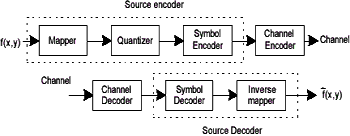
Figure 1 General compression system model
The principle of the error-free compression strategies, it normally provides the compression ratio of 2 to 10. Moreover, they are equally applicable to both binary and gray-scale image. The error-free compression techniques generally composes of two relatively independent operations: (1) modeling, assign an alternative representation of the image in which its interpixel redundancies are reduced; and (2) coding, encode the representation to eliminate coding redundancies. These steps correspond with the mapping and symbol coding operation of the source coding model.
The simplest approach of error-free image compression is to reduce only coding redundancy. Coding redundancy normally presents in any natural binary encoding of the gray levels in an image and it can be eliminated by construction of a variable-length code that assigns the possible shortest code words to the most probable gray levels so that the average length of the code words is minimized.

where
L is the number of gray levels.
rkrepresents the gray levels of an image.
l(rk) the number of bits used to represent each value of rk.
pr(rk) probability of rk occurring.
The modeling part can be formulated as an inductive inference problem. Having scanned past data ix=x1x2x3… xi, one wishes to make inference on next pixel value xi+1 by assigning a condition probability distribution p(.|xi) to it. Ideally, the code length contributed by xi+1 is –log p(xi+1|Xi ) bit, which averages to the entropy of the probabilistic model. Assigns a high probability value to the next pixel with skewed (low- entropy) probability distribution is desirable. It can be obtained through the larger conditioning regions or context and generally broken into the following components:
- A prediction step, in which a deterministic value xis guessed for the next pixel xi+1 based on past sequence xi(a causal template)
- The determination of a context in which xi+1 occurs.
- A probabilistic model for the prediction residual (error signal) conditioned on the context of xi+1.
Transform Image
In the baseline system, it is often called the sequential baseline system, the input and output data precision are limited to 8 bits, whereas the quantized DCT values are restricted to 11 bits. The compression itself is performed in three sequential steps: DCT computation, quantization, a variable-length code assignment. The image is first subdivided into 8x8 blocks pixel. Subimage is encountered, its 64 pixels are level shifted by subtracting the quantity 2n-1, where 2nis the maximum number of gray levels. The 2-D discrete cosine transform of the block is then computed, quantized and reordered, to form a 2-D of quantized coefficients.
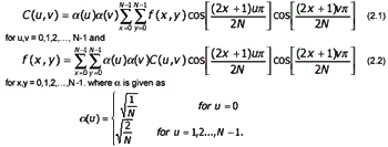
The remapped 2-D of quantized coefficients which is generated by mapping the pixel (i,j) of subimage (u,v) to subimage (i,j) with pixel (u,v) that easily done by interchange between index of subimage and pixel for 64*64 pixel image.
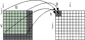
Figure 2 Transformed coefficient mapping
The Rice-Golomb coding procedure is designed to take advantage of the long runs of zeros that normally result from the reordering. The nonzero coefficients are coded using a variable-length code.

Figure 3: Simplified diagram of proposed encoder.
Context Based Lossless compression
1. Prediction
The prediction and modeling units in (Weinberger, 1996) are based on the causal template, where x denotes the current pixel, and a, b, c and d are neighboring pixel as shown in the Figure 4.
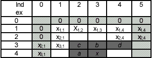
Figure 4 Preassigned pixels and causal template for context modeling and prediction
The inner box represents the actual image, while the shaded area represents the implied values for Rb, Rc and Rd when the sample Ix is in the first line, for Ra and Rc when the sample Ix is in the first column, and for Rd when the sample Ix is in the last column. From the values of the reconstructed samples at a, b, c and d, the context first determines if the information in the sample x should be encoded in the regular or run mode:
- The run mode is selected when the context estimates that successive samples are very likely to be either identical. The context modeling procedure selects the run mode and the encoding process skips the prediction and error encoding procedures. In run mode, the encoder looks, starting at x, for sequence of consecutive samples with values identical to the reconstructed value of the sample at a. This run is ended by a sample of a different value or by the end of the current line, whichever comes first. The length information, which also specifies one of the above two run-ending alternatives, is encoded using a Golomb coding.
- The regular mode is selected when the context estimates samples are not very like to be identical. The predictor combines the reconstructed values of the three neighborhood samples at position a, b, and c to form a prediction of the sample at position x as shown in Figure 3. The error prediction is computed as the difference between the actual sample value at position x and its predicted value. This error prediction is then corrected by a context-dependent term to compensate for systematic biases in prediction. The corrected error prediction is then encoded using a derived procedure form Golomb coding.
The first step in the context determination procedure shall be compute the local gradient values, D1, D2, D3 of the neighborhoods in the following:

The next step is mode selection, if the local gradients are all zero the encoder shall enter the run mode, otherwise the encoder shall enter the regular mode. The local gradient quantization and merging will be preformed by using the non-negative thresholds T1, T2 and T3 to obtain the vector (Q1, Q2, Q3) representing the context for the sample x.
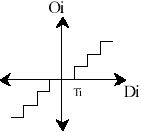
Figure5. A threshold coding quantization curve.
3. The edge-detecting predictor
To estimate Px of the value at the sample of x, the using encoded shall be determined from the values Ra, Rb and Rc at the positions a, b, and c by the following condition,

The predictor can be interpreted as picking a in many cases where a vertical edge exists left of the current location, b in many cases of an horizontal edge above the current location, or a plane predictor a+b-c if no edge has been detected.
4. The prediction correction
After Px is computed, the prediction shall be corrected according to the sign of context vector (Q1,Q2,Q3) with the prediction correction value C[ Q], it is derived from the bias cancelation procedure.

Then, the prediction error can be computed and encoded by Golomb’s coding.

5. Rice-Golomb Coding
The special case of Golomb codes with m=2kchoosing m to be a power of 2 leads to very simple encoding/decoding procedures: the code for n ³ 0 consists of the k least significant bits of n, followed by the formed number by the remaining higher order bits of n, in binary representation. The length of the encoding is k+1+[ n/2k]

Fig 6. The example of Rice-Golomb coding
In order to find k for Golomb coding, the encoder and decoder maintain two variables per context: N, a count of prediction residuals seen so far, and A, the accumulated sum of magnitudes of prediction residuals. The coding parameter k can be computed by

Results
Figure7 shows the two different continuous tone images, were transformed to DCT coefficient and remapped. The first image is flatter than the second one. The corresponding transformed coefficients are shown in same way. To increase the continuous of coefficients can be done by remapping procedure as shown in Figure (b) and (c).
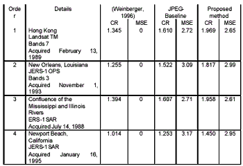
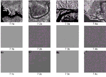

For the high continuous tone image, the compressed image sizes seem not difference in three method and evidently observe when compared with the low continuous tone image.
Conclusion
The proposed method has taken the advantages of both transform and context based compressions. The DCT transform can reduce the interpixel redundancy, while context based Rice-Golomb coding offers the high reduction of coding redundancy. This proposed method shows the performances as high as continuous level that will degrade the compression ratio when applies with the previous method (Weinberger, 1996) or JPEG-baseline.
References
- Weinberger, M. J., 1996. LOCO-I: A low complexity, context-based, lossless image compression algorithm, pp.140-149.
- Gonzales, R. C., 1993. Digital Image Processing, Wesley Publishing Company.
- Golumb, S. W., 1966. Run-length encodings, Vol. IT-12, pp.399-401.
- Rice, R. F., 1979. Some practical universal noiseless coding techniques. In: Jet Propulsion Laboratory, Pasadena, CA, U.S.A., Rep. JPL-79-22.