| GISdevelopment.net ---> AARS ---> ACRS 2002 ---> Data Processing, Algorithm and Modelling |
Knowledge based object
extraction technique
Mohamed
Abdel-salam
PhD candidate & Research Assistant
Department of Geomatics Engineering, The University of Calgary
2500 University Drive N.W.
Calgary, AB, T2N 1N4, Canada
Email: mabdel@ucalgary.ca
Phone +1 (403)-282-9308
Fax +1 (403)284-1980
PhD candidate & Research Assistant
Department of Geomatics Engineering, The University of Calgary
2500 University Drive N.W.
Calgary, AB, T2N 1N4, Canada
Email: mabdel@ucalgary.ca
Phone +1 (403)-282-9308
Fax +1 (403)284-1980
Abstract
Since the beginning of remote sensing technology, bottom up methods for interpretation of scenes monopolize remote sensing activities. For example, in the conventional per-pixel classification, which is a bottom up approach, the system uses the information hidden in spectral data only. Such techniques suffer from drawbacks caused by mixed pixels and spectral overlap. Knowledge about objects, sensor and environment is hardly considered. Therefore a lot of problems appear in the conventional methods are related to insufficient representation of the available knowledge. The difference between human interpretation and any computer assiste d image analysis is that humans use spatial information like texture, shape, shade, size, site, association and topology, while computers are powerful in handling the gray values in the image. In this paper a new technique for object recognition and identification is proposed. The proposed technique employs knowledge about objects and edge spread function. These two types of knowledge are hardly included in the conventional methods. The heart of proposed technique is the integration of the existing knowledge and numerical optimization techniques. A new proposed cost function, which is used by the optimizer, and a rectangular class of objects have been studied in this paper. The high performance of the method is clearly shown in the obtained results. Varieties of objects have been extracted with the proposed method some of them as will be shown are almost impossible for bottom up approach.
Introduction
Bottom approaches for remote sensing data interpretation use only spectral knowledge represented in pixels. Other existing knowledge in the scene is not considered at all. These exiting knowledge can be categorized into three main branches. The first branch is related to the object: geometric and radiometric. The second branch is related to the sensor: imaging technique, bluer model, noise model, image acquisition model and projection model. The third branch is related to the environment: path and illumination model (Mulder and Fang, 1994), (Van der Heijden, 1994). For most farms, the agriculture fields enjoy certain shapes and border thickness, and even orientations. Integrating this simple existing knowledge in the interpretation process can enhance the outcome. The way to integrate different types of knowledge in known as model based image analysis. It is popular in different areas like industrial applications, medical applications and computer vision. It tries to model a scene in terms of objects and parameters and then it estimates these parameters. Therefore, using model based approach for interpreting imagery can be powerful.
Proposed Technique
The proposed technique starts with the initiation of a hypothetical object model and it checks the corresponding statistical information of the multispectral information inside this object. Based on this statistical characteristic, the object parameters are adjusted through a numerical optimizer till a given satisfactory statistical criterion is satisfied. This criterion acts as a cost function. Then the object will be stored as identified object. The method will start again to search for another object, avoiding the positions of the previous objects.
- Object Model
A rectangular shape class is used in this paper. The rectangular-shape class is five parameters primitive. Its parameters are locations (two parameters), length of the rectangular primitive, width of rectangular primitive and the orientation of the primitive.
- Edge Spread Function (ESF) Model
Pixels at boundaries are among the major causes of uncertainty of object boundaries that lead to inaccurate parameter estimation of objects from remotely sensed data. Two issues are related to the edge-spread function: how to model it and how to include it. It is assumed that the edge-spread function is a piecewise linear function of a certain width. The edge-spread function is assumed to be symmetry independent of the orientation of the edge. Compensating the effect of ESF is based on detection of the optimum size of the Hypothetical object and then the hypothetical object size is increased by half the width of the edge-spread function in each direction
- The Proposed Objective (Cost) Function
Cost, objective, function expresses the consistency of a hypothesis with the truth. It should reflect big value if the hypothesis wrong and small value if the hypothesis true. In most model-based techniques, pixel classification results are the cost function parameters. The dependence of cost function on classification should be avoided since classification procedure is subjective. In this paper a new cost function is proposed. The standard deviation of the mean (StdM), the normalized standard deviation (NStd), and the Std are candidates as objective functions. Therefore, the only prior knowledge taken into account is that different objects in the image show a contrast. No knowledge about the radiometric distribution is necessary. The Std tends to make the object as small as possible; therefore, it can’t be a cost function. Standard deviation of the mean is a well-known quantity in observation and measuring samples. StdM and NStd depend on the both the population variance and sample size. One reason for choosing these objective functions is that they tend to enlarge homogeneous objects as much as possible. The average of the cost function in the three bands is used. In the following the equations of NStd are given.
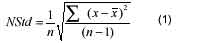
where:
x : is the digital number, n is the number of pixels
is the mean of the digital number inside the hypothetical object
The StdM is comparable in its performance to normalized Std. The normalized Std has the same behaviour of StdM, but NStd is not sensitive toward the noisy parts like the StdM. So the selection of StdM is suitable for the current problem and this is validated by real data.
- The Optimizer
Model based image analysis needs a huge amount of calculations. The exhaustive search method, which evaluates all possible combination of the parameter values, is time consuming. It is not realistic for large problems. To overcome this problem, optimization is used. Optimization starts with an objective function and a set of initial parameters and the goal is to find the set of parameters that gives the optimal objective value (Gile,1997). The optimal objective value of the objective function is problem dependent. Two types of optimizers used in this technique are: the Steepest Descent and Simplex method (McKeown,1990).
Several experiments with real data are implemented. These experiments are divided into two main categories; the first category deals with scenes consisting of rectangular shapes only, while the second x.category deals with scenes consisting of rectangular shapes in addition to other shapes. For numerical optimization, gradient information, steepest descent optimizer, is used at the beginning to move the initial parameters to a good location, a low cost area, then different simplex iterations deliver the result to each other. The simplex iterations start work by beginning with population, initial values, of a big step and ending with population with a small step. The reason for this is to overcome local minima as much as possible.
1. Scenes with Rectangular Shapes Only
Three different scenes are selected. The first scene (154x172 pixels) consists of two different objects, the second (114x107) consists of three objects with the same crop type and the third (373x342) contains six objects with three different crops. The scenes are shown in figure (1). Before going to further processing it is necessary to obtain information about the width of the edge spread function. Since there is no information available about it, the edge-spread function is assumed to be a piecewise linear symmetrical function. A width of three pixels is selected for edge spread function. This value is used in the real data experiments. It should be noted that experiment 1 and 3 contain an object with a repeated pattern texture, a glass house, which is a problematic issue in bottom up approaches. Fig (1) shows an example of the output of our MBIA algorithm. The figure shows an automatic overlay of DXF layer that contains the extracted object and the input image. In addition to the DXF layer, the algorithm produces five geometrical parameters for each object.
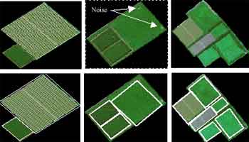
Figure (1) Result of real data (scenes with only rectangular shapes)
The results of the three experiments show that the method detected and extracted the existing objects. Some error appears in experiment 1 due do inaccurate modeling of ESF (the given value of ESF width was too big). In experiment 2, the existence of noise near the corners makes one of the objects to be extracted with some error. The reason is that the optimizer could not overcome the local minimum due to this noise. In experiment 3 the overlaying of the extracted objects by the image shows that all objects are extracted successfully. Only the green house object is too large. The reason is that the similarity between the glasshouse and the surrounding which makes both of them appear as one object. The similarity is mainly, between the neighbor object and one of the textures that construct the glasshouse.
2. Irregular Shapes
To consider agriculture fields as only rectangles is hardly realistic. The existence of irregular shapes beside the rectangular shapes is more probable. In this section a method for detection of only rectangular shapes from a scene is explained. Considering an irregular shape as shown in figure (2) left, Noise.until now the proposed method will try to find a rectangle with minimum cost inside this irregular shape. For example consider the solid rectangle, candidate object, as identified object inside the actual irregular object. This object should be rejected. The rejection method is based on the detection of any irregular extension of the candidate rectangle. Studying the two hypothetical thin objects (ob1 and ob2), it is evident that Ob2 has lower cost value compared with Ob1. The reason is that since an object is homogeneous, increasing the size of the object reduces the cost function value. This previous remark is considered the criteria for rejection of an irregular object. To reject a rectangle, in other words not to extract a candidate rectangle with minimum cost function, several hypothetical thin rectangles inside and just outside this candidate object are checked. Figure (2) right shows the checks location. Since we are interested in detecting any small amount of change across the border, the StdM as cost function for check is more convenient in this case.
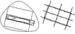
Figure 2 Irregular shapes rejection strategy and checks locations
The parameters of those thin rectangles depend on the definition of the rectangular shape. In the current context the rectangular shape is identified as any candidate rectangle (with minimum cost function) and satisfies the following properties.
- (Couple of hypothetical thin rectangles (like object1, 2)) |CF object 1 < CF object 2.
- The extensions of these thin objects are 20% of the dimension of the candidate rectangle.
- The width of the thin object is 0.2 of the width of the candidate rectangular in other words we can say that the algorithm performs the following steps:
- Chooses a number of small strips such that the extracted rectangle is covered.
- Extends each strip with 20% over the boundary of the rectangle. Do this for both sides of the strip.
Scenes with Rectangular Shapes in Addition to non Rectangular Shapes
Three different scenes are used in this stage. The first scene contains only one rectangle. The second one contains two rectangles; the third one contains three rectangles. The edge spread function width adopted in these scenes is 1.5 pixels. Figure (3) shows that the entire expected rectangular object was successfully detected and extracted. One more object (the third object in third experiment) was expected to be detected; the object fails to satisfy the rules of the rectangular shapes. The reason for that is the existence of a homogeneous zone near the end of the object, which considers extension for the object.

Figure 3 Results of second type of scenes
Analysis of the results
A twofold criterion is used to analyse the result. It is qualitative in terms of number of extracted objects compared to the number of actual objects in the scene and the running time and quantitative in terms of numerical figures, which describe the results. The qualitative result of the experiments shows that the technique identified all expected rectangles in the scenes. Only one rectangle was expected to be extracted in the third experiment of the irregular shapes and later this rejection is explained. This object was not concordant with the rules that define the rectangular shapes. The running time as component of qualitative assessment points out that the Matlab code is not optimised and it is time consuming. The quantitative component of the assessment is explored in the following sections.
1. Method of quantitative evaluation
To evaluate quantitative success of the procedure, we have to find truth data to assess the results. To do that the images that are us ed in the experiments are digitised using on screen digitising. The digitising is done in Arcview (GIS software). The delineating of boundaries is done in such a way that it is as close as possible to the reality. It is necessary to say that subjectivity and human delineating errors are inevitable. The extracted objects are overlaid by the output of on screen digitising. After overlying the results and the truth data, Arcinfo (GIS software) is used to process the data. Arcinfo is mainly used to build topology and to calculate the overlapped area. Mainly three quantities are measured; wrongly predicted parts, parts not predicted, and correctly predicted parts as shown in figure 4. These measurements are done for each object for each test. The chosen quantita tive criterion for assessment is twofold. The first is related to correctness of extraction and the other relates to the error in extraction. For the first part the correctness in extraction is considered as the ratio between the correctly extracted areas to the area of the digitised object. The second part, which is related to the error in extraction, is divided into two subparts. The first subpart is the ratio of the wrongly predicted area to the.digitised area; the second subpart is the ratio of the not predicted part to the digitised area. It should be clear that the summation of the three quantities does not produce 100% because these ratios are normalised by the digitised area. The three quantities: the ratio of correct prediction, the ratio of wrong prediction and the ratio of the not predicted parts are 97.01,7.56, and 2.99% respectively for the six experiments.
Figure 4 Assessment procedures
This paper has introduced a method for geometrical object parameter estimation of model shapes from multispectral images. A rectangle model shapes is used. The paper presents a new cost function. The cost function avoids the problems of using training data in the extraction of agriculture fields. The nature of the cost function makes the technique independent of assuming any radiometric distribution of the agriculture field. The output results of several scenes show that the method can detect and extract the objects with high accuracy. The output of the technique is easy to integrate with GIS. It is produced in two forms, the first is DXF file and the second is the five parameters of each object. ACKNOWLEDGEMENTS This work was done under the Netherlands fellowship program, at ITC, the Netherlands. ITC is deeply appreciated.
References
- Gile, E., Murray, W., Wright, H. 1997. Practical Optimization, Academic Press, Great Britain
- Van der Heijden, F., 1994. Image Based Measurement Systems: Object Recognition and Parameter Estimation, Wiley & Sons, Great Britain - ISBN 0-471-95062-9.
- McKeown, j. j., 1990. Introduction to unconstraint optimisation. IOP publishing Ltd., Great Britain. 122p, ISBN 0-7503-0025-6.
- Mulder, N. J. and Fang, L. 1994. Knowledge based image analysis of agricultural fields in remotely sensed images. Pattern recognition in practice: Vol. IV , pp. 197-211