| GISdevelopment.net ---> AARS ---> ACRS 2000 ---> Water Resources |
Groundwater Level Forecasting
with Time Series Analysis
Miao-Hsiang PENG and
Jin-King LIU
Energy and Resources Laboratories, ITRI, Hsin-Chu, TAIWAN
E-mail: 781062@itri.org.tw ; JKLiu@itri.org.tw
Tian-Yuan SHIH
Professor, Department of Civil Engineering, National Chiao-Tung University,
Hsin-Chu, TAIWAN
E-mail: tyshih@cc.nctu.edu.tw
Key Words:Energy and Resources Laboratories, ITRI, Hsin-Chu, TAIWAN
E-mail: 781062@itri.org.tw ; JKLiu@itri.org.tw
Tian-Yuan SHIH
Professor, Department of Civil Engineering, National Chiao-Tung University,
Hsin-Chu, TAIWAN
E-mail: tyshih@cc.nctu.edu.tw
Autocorrelation Function, ARIMA Model, Land Subsidence, Stochastic Process, Stationality
Abstract:
This study investigates the application of time series analysis methods for forecasting groundwater levels. The study site is located in western Taiwan where serious land subsidence has occurred. A series of monthly groundwater level observations made during the period 1993 and 1999 is used for the experiments. Univariate time series models, including ARIMA models and the time series decomposition method, are applied and the resulting accuracy is compared. Empirical results indicate that groundwater level data series in this study are cyclical. ARIMA models generate more accurate forecasts. The forecasting of ARIMA models presents the characteristics of trend and seasonal variation.
1. Introduction
Groundwater level models provide useful information for land subsidence forecasts. The Univariate Box-Jenkins (UBJ) ARIMA analysis (Box, Jenkins and Reinsel, 1994) has been used in many applications, such as medical, environmental, financial, and engineering applications (Abdel-Aal and Mangoud, 1998; Kumar and Jain, 1999; Mitosek, 2000). A comparative study between ARIMA models and the time series decomposition model for forecasting groundwater levels is discussed in this article.
2. Site Description and Data Collection
Records of groundwater levels were compiled for wells in a monitoring network in the Cho-Shui alluvial fan near southwest Taiwan, starting around 1993. Groundwater-levels were generally measured once a month.
3. Arima Modeling of the Groundwater Level
The statistical package MINITAB for Windows is employed to develop the ARIMA models. There are four stages in the modeling process (Bowerman and O'Connell, 1993), i.e. identification, estimation, diagnostic checking, and forecasting.
3.1 Identification
The first step is to plot the data for the monthly groundwater-level time series for 7 years (Figure 1). Data for the first 5 years are used for constructing the ARIMA model and the remaining years are reserved for evaluation. A simple linear regression model is used to characterize the trend component. The result of regression analysis is shown in Table 1. The trend of the overall groundwater-level develops through time. A clear seasonal pattern, with low levels from November to April and high levels from February to August, emerges from the data gathered.
| Site | Intercept (m) | Slope | Mean absolute deviation (m) | Mean squared deviation (m) |
| IWu | -28.2856 | 0.0635 | 2.61 | 3.22 |
The first insight into the statistical properties of the time series is shown in Table 2. Performing the first differencing on the groundwater-level series reduces the series mean from -25.46 to 0.03. The first differencing often results in a stationary mean value of approximately zero (Figure 2).
| Data | Max (m) | Min (m) | Mean (m) | Variance |
| Raw | -16.95 | -31.98 | -25.46 | 11.852 |
| First differencing | 5.21 | -7.60 | 0.03 | 5.478 |
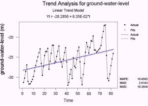
Figure 1. Monthly groundwater-level data and regression model.
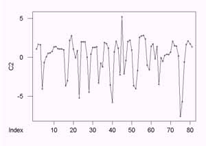
Figure 2. First differencing sequence plot.
To remove seasonal nonstationarity of the series, the first seasonal differencing is applied:
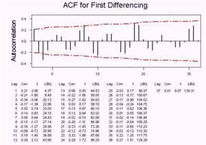
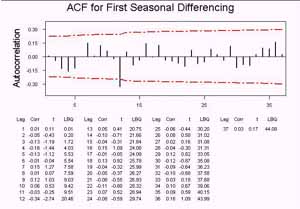
Wt = Et - Et-1 - Et-12 + Et-13; t=14,15,… (1) Where Wt is the first seasonal differencing of ground-water level Et . A spike at the first seasonal lag 12(|t-value|>1.6) appear on both acf and pacf (Figure 4), indicating that the period of differencing is 12 months.
 |
 |
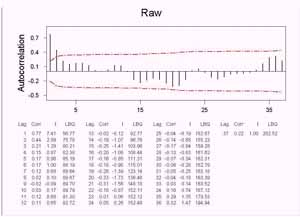
(a) the raw monthly time series;
(b) the time series obtained through the first differencing
 |
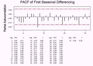 |
Figure 4. The autocorrelation function (ACF) and the partial autocorrelation (PACF) for the time series obtained from the first seasonal differencing.
3.2 Estimation
The parameters for each model are estimated with the ARIMA module of MINITAB. The results are summarized in Table 3. The constant terms of all cases are negligibly small since the modeled differencing series has a nearly zero mean. The good quality of the coefficients are significantly greater than zero (|t-value|>2.0) and satisfy the stationarity conditions. Absolute values for all coefficients are also significantly different from 1.
| Model | Parameter | Coefficient | St. Dev. | t-value |
| ARIMA(0,1,1)(1,1,0)12 | MA1 | 0.0028 | 0.1144 | 0.02 |
| SAR12 | -0.5768 | 0.1065 | -5.41 | |
| CONSTANT | 0.0008 | 0.2594 | 0.00 | |
| ARIMA(1,1,0)(1,1,0)12 | AR1 | -0.0021 | 0.1144 | -0.02 |
| SAR12 | -0.5727 | 0.1066 | -5.37 | |
| CONSTANT | 0.0006 | 0.2602 | 0.00 | |
| ARIMA(1,1,1)(1,1,1)12 | AR1 | -0.1016 | 0.8447 | -0.12 |
| MA1 | -0.2270 | 0.8162 | -0.28 | |
| SAR1 | -0.3225 | 0.1149 | -2.81 | |
| SMA1 | 0.9192 | 0.0850 | 10.82 | |
| CONSTANT | -0.03478 | 0.03617 | -0.96 | |
| ARIMA(1,1,1)(1,1,0)12 | AR1 | 0.8036 | 0.0765 | 10.50 |
| MA1 | 0.9794 | 0.0431 | 22.74 | |
| SAR12 | -0.6026 | 0.1058 | -5.70 | |
| CONSTANT | 0.00479 | 0.01086 | 0.44 | |
| ARIMA(1,1,0)(0,1,1)12 | AR1 | 0.1014 | 0.1173 | 0.86 |
| SMA12 | 0.8729 | 0.0980 | 8.91 | |
| CONSTANT | -0.00998 | 0.05413 | -0.18 | |
| ARIMA(0,1,1)(0,1,1)12 | MA1 | -0.1158 | 0.1157 | -1.00 |
| SMA12 | 0.8631 | 0.0969 | 8.90 | |
| CONSTANT | -0.00907 | 0.06239 | -0.15 |
3.3 Diagnostic checking
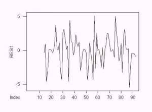
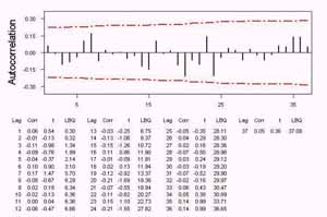
The statistical adequacy of the estimated models is then verified. The ACF function for the residuals resulting from a good ARIMA model will have statistically zero autocorrelation coefficients. Figure 5 shows a plot of the residuals for ARIMA(1,1,0)(1,1,0)12 model. The residual plot shows small variations around the zero mean. The plot of the estimated residual ACF in Figure 5 indicates that there is no significant autocorrelation, and the model adopted will be acceptable.
3.4 Forecasting
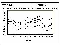
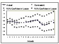
Two ARIMA models were applied to forecast the 21 water level values from January 1998 to September 1999. The forecasts are then compared with the measured data. The forecasted time series and its 95% confidence level error bound are plotted in Figure 5 for both models. It is observed that all measured monthly values fall within the error bound, and the forecasts track the seasonal pattern reasonably well.
 |
|
 |
|
(a) the ARIMA(1,1,0)(1,1,0)12 model;
(b) the ARIMA(1,1,1)(1,1,0)12 model.
4. Comparison with various Modeling Techniques
Three accuracy indices are computed for six ARIMA models and the decomposition model. As shown in Table 4, the ARIMA(1,1,1)(1,1,1)12 model has mean absolute error 2.29m and mean square error 8.33 m2, and is ranked the lowest among all.
| Model type | Mean absolute error (m) | Mean square error (m2) | Maximum absolute error(m) |
| ARIMA(1,1,1)(1,1,1)12 | 2.29 | 8.33 | 4.86 |
| ARIMA(0,1,1)(1,1,0)12 | 2.84 | 10.24 | 5.28 |
| ARIMA(1,1,0)(1,1,0)12 | 2.54 | 10.25 | 5.28 |
| ARIMA(1,1,1)(1,1,0)12 | 2.86 | 11.30 | 6.34 |
| ARIMA(1,1,0)(0,1,1)12 | 2.75 | 12.15 | 6.58 |
| ARIMA(0,1,1)(0,1,1)12 | 2.84 | 13.25 | 7.06 |
| Decomposition | 3.22 | 12.02 | 5.22 |
5. Conclusions
The multiplicative combinations of nonseasonal and seasonal ARIMA models have been used to forecast groundwater-levels for land-subsidence areas, located in southwest Taiwan. The forecasting performance of the ARIMA models presents a seasonal trend. The various ARIMA models forecast monthly data for the evaluation with a mean error of about 2.3m to 2.9m. In terms of numerical accuracy measures, the ARIMA model generates more accurate forecasts than the decomposition model. It should be emphasized that the objective is not to determine which forecasting method is the best, but to introduce the various procedures available to check the forecasting.
References
- Abdel-Aal, R.E. and Mangoud, A.M., 1998. Modeling and forecasting monthly patient volume at a primary health care clinic using univariate time-series analysis. Computer Methods and Programs in Biomedicine, 56, pp.235-247.
- Bowerman, B.L. and O'Connell, R.T., 1993. Forecasting and Time Series: An Applied Approach, Duxbury Press, Belmont, CA.
- Box, G.E.P., Jenkins, G.M. and Reinsel, G.C., 1994. Time Series Analysis, Forecasting and Control, Prentice Hall, Englewood Cliffs, N.J.
- Kumar, K. and Jain, V.K., 1999. Autoregressive integrated moving averages (ARIMA) modeling of a traffic noise time series. Applied Acoustics, 58, pp283-294.
- Mitosek, H.T., 2000. On stochastic properties of daily river flow processes. Journal of Hydrology, 228, pp188-205.
- Thury, G. and Witt, S.F., 1998. Forecasting Industrial Production Using Structural Time Series Models. Omega Int. J. Mgmt Sci, 26, pp751-767.