| GISdevelopment.net ---> AARS ---> ACRS 2000 ---> Water Resources |
Using Spectral Mixture
Modeling Techniques to derive Land-Cover parameters for Distributed
Sediment Yield Estimation
Enrico C
PARINGIT1 and Kazuo
NADAOKA2
1Graduate student, 2 Professor Department of Civil Engineering
Tokyo Institute of Technology
2-12-1 O-okayama, Meguro-ku, Tokyo 152-8552,
E-mails: ecp@mei.titech.ac.jp , nadaoka@mei.titech.ac.jp
Tel: (81)-3-5734-3486 Fax: (81)-3-5734-2650
Japan
1Graduate student, 2 Professor Department of Civil Engineering
Tokyo Institute of Technology
2-12-1 O-okayama, Meguro-ku, Tokyo 152-8552,
E-mails: ecp@mei.titech.ac.jp , nadaoka@mei.titech.ac.jp
Tel: (81)-3-5734-3486 Fax: (81)-3-5734-2650
Japan
Key Words:
Sediment yield estimation, spectral unmixing, leaf area index
Abstract:
Vegetation and soil properties and their associated changes through time and space affect the various stages of erosional processes. This paper discusses the application of remote sensing techniques in the retrieval of vegetation and soil parameters necessary for the distributed soil loss modeling in small agricultural catchments. To account for the compositional nature of the ground surface as depicted on remotely-sensed data, a linear spectral mixture modeling (LSMM) approach is used to parameterize vegetation and soil optical properties. Results of these parameter estimates were coupled to a DEM-based distributed hydrologic rainfall-runoff model to simulate overland flow and sediment yield for a given rainfall event. Field observations were undertaken to gather spectral and physical measurements of vegetation and to obtain data for soil hydraulic properties. Results of the sediment yield model indicate strong relationship between vegetation abundance and erosion by soil detachment. A general agreement between the simulated and measured sediment discharges is also observed. The method provides a physical basis for incorporating the spatial and temporal variability of various vegetation and soil condition to dynamic processes such as soil erosion and may be applicable to monitor other non-point source pollutants from agricultural watersheds.
1. Introduction
The risk of soil erosion by water, varies as a function of many factors, but the degree of protection provided by vegetation is one of the most important. Usually erosion rates are computed by means of empirical methods or if treated in terms of physically-based models, are highly idealized, such that effects of vegetation presence become trivialized, mainly due to its high spatial and temporal variation. Leaf area index (LAI) and percentage vegetation cover (PVC), two parameters routinely derived from remote sensing, can provide the necessary details to incorporate vegetation effects to soil losses.
Spectral mixture models are among the popular methods to resolve the optical components of surfaces with diverse land cover types especially useful when the analysis is constrained by the spatial resolution of the available dataset (van Leeuwen et. al, 1997). A desirable feature of mixture models is that they are able to estimate the fractional abundance of vegetation and soils simultaneously, appropriate for purposes which require both information at the same instant such as in the case of erosion analysis. LSMM is most appropriate for crop plants since leaves are relatively dominant, soil reflectance is uniform, topography is minimal and most crowns can be modeled with simple geometric shapes, the favorable conditions to achieve linear spectral mixing.
This study was conducted to investigate the effect of applying vegetation indexes, particularly LAI and PVC, obtained through spectral mixture analysis of remotely-sensed data, to quantify soil losses, particularly sediment discharge from a predominantly agricultural area during rainfall events with consideration to development stage of vegetation.
2.Materials and Methods
2.1 The Study Area
A small catchment test area (11 km2) was chosen to exemplify the essential points of this research. The study area represents a typical tropical environment prone to high degree of rain-induced erosion. It covers the eastern portion of Ishigaki, an island south of the main Okinawa Island Prefecture in Japan. It is located about 24º23' N latitude, 124º14' E longitude, with topography varying from flat, undulating to hilly terrain currently being subjected to intense agricultural cultivation. Crops consists mainly of tobacco, sugarcane, rice and pineapple. The area is drained through the Todoroki River with outlet to the coastal area, where a special concern is focused on mitigating the effects of sediment discharge on coral reef zones (Dikou and Takeaki, 1999).
2.2 Remote Sensing and Field Observation Data
Field campaigns were conducted on three occasions: early June, early August and early September with various inland data-logging instruments to measure river discharge, turbidity, depth and rainfall in different locations inside the watershed. Spectral signatures for both soil and vegetation were also gathered to parametrize reflectances from 320 to 1080 mm range. Water samples have been previously obtained for turbidity-sediment concentration calibration of the instruments. Soil samples were processed in the laboratory to obtain various hydrologic parameters such as hydraulic conductivity, soil moisture, porosity, grain size and typing. Vegetation structure measures such as plant spacing, layering and leaf dimensions were also recorded.
Due to the absence of remotely-sensed data, both spaceborne and airborne, within the period of field observations, the land cover captured from the aerial photographs taken in 1995 was assumed to be the prevailing land surface condition. The use of an asynchronous data can be justified since the dates of the aerial photography lie within the same season of the year and that no major changes in cropping patterns and infrastructure developments has occurred since.
2.3 Spectral Mixture Modeling of Vegetation and Soil
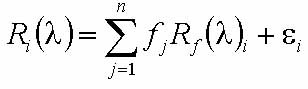
Spectral unmixing is a deconvolution technique that aims to decompose the mixed reflectance spectrum, Ri(l) of a ground element in an imagery into landcover components based on the LSMM (Settle and Drake, 1993) given by:
and
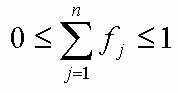
(1), (2)
where Rf(l) is reflectance of end-member spectrum of a homogenous land cover for each band i of n land cover types, and ei is the residual noise. The objective is to estimate , for each land cover component within a pixel by inversion technique, a typical solution of which is the classical least squares approximation, in matrix notation,
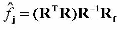 However, since there
is a constraint to sum up the fractional cover to one by Eq. (2), then a
Lagrangian formulation gives the more appropriate solution:
However, since there
is a constraint to sum up the fractional cover to one by Eq. (2), then a
Lagrangian formulation gives the more appropriate solution: 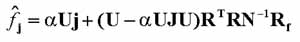
(3)
where the U=RTN-1R, a =(jTUj)-1, J (=jjT) is an n x n identity matrix of n x 1 js with elements =1 consisting of and N represents the sensor noise characterized by the variance-covariance matrix. The equivalent f for the soil and vegetation cover are used as the values percentage soil cover (PSC) and PVC respectively. PVC quantifies merely the portion of exposed canopy. In hydrologic modeling as will be shown later, it becomes more important to determine the fractional abundance or sparsity of vegetation, which can be adequately described by LAI. The reflectance model of Gilabert et al. (2000) is modified obtaining:
(4)
C is regarded as a weighing parameter assumed to be invariant with wavelength and assumes complete absorption. Its value rather, varies with angle of light source and plant architecture. An immediate application of LAI is to compute for the interception capacity of a particular canopy for rain expressed as a function of the LAI given by:
(5), (6)
where Sr is the canopy interception capacity (m), Sr0 and LAI0 are the maximum canopy interception capacity and leaf area index (m2 m-2) respectively specific for each vegetation type.
2.4 Runoff Modeling and Sediment Routing
The overland flow runoff routing model utilizes the DEM (digital elevation model)-based diffusion wave equation according to the procedure outlined by Wang and Hjelmfelt (1998) while the sediment yield component is taken from SHESED model of Wicks and Bathhurst (1996). Both models are ideal for small flat watersheds where the main processes affecting sediment yield are soil erosion by raindrop impact and overland flow and sediment transport by overland and bed channel flows. The results of the PVC and PSC computations may be used on the following expression:
(6)
where DR is the soil detached by raindrop impact (kg m-2 s-1), Kr is the raindrop soil erodibility coefficient varying according to the type of soil, Fw is the water depth correction factor, while MR and MD are momentum squared for raindrop and leaf drip respectively. Values or the expressions to obtain Kr, Fw, MR and MD may be taken from Wicks and Bathhurst (1996) and is still subject to calibration. Application of unmixing results to Eqs. (5) and (6) allow attribute variability within one pixel unafforded in other routing techniques.
2.5 Data Processing and Hydrologic Modeling Steps
The spectral signatures for six full-grown vegetation and three soil types were average-sliced into three ranges equivalent to the spectral sensitivity of a colour film with a minus-blue filter. Thirteen aerial photographs were scanned, registered to a 1:25,000 topographic map at 10 m resampling, and mosaicked, with correction for vignetting effects. Radiometric calibration was performed by obtaining coefficients from fitting the RGB values of homogenous landcover types with their equivalent sliced signatures. These coefficients were then applied to the whole 440 x 445 pixel data to generate the radiance image. The sliced signatures also served as values for Rf, the "pure" end-member spectra.
In the unmixing proper, applying the appropriate crop and soil type signatures is determined through the use of agriculture land use and soil series maps with validation for soil sampled from the field. Other field data such as leaf dimensions and number, and plant height, spacing and density for each full grown crop served as an input to compute their respective LAI0s while values for C were obtained from Gilabert et al.(2000) but may be obtained if leaf samples are brought to the laboratory for an LAI experiment. Built-up areas and bare soil types were masked out and automatically assigned LAI0s of zero. Selective LAI0 and C usage likewise makes use of the agriculture land use map.
The DEM and channel routes were obtained by the digitizing the topographic map while data from the four rain gauges were used to generate a continuous distributed rainfall map for four rainfall events by inverse distance interpolation. The hydrologic model was then implemented in computational grid size of 10 meters at 10-second time intervals inside the watershed boundary. Aside from the Courant-Friedrichs-Lewy (CFL) routing scheme stability criterion, the selection of grid size and time interval depended on the consideration for an ideal grid size that minimizes detail loss due to spatial aggregation while maintaining a manageable number of cells for optimal computation time. It is assumed that for a single grid cell, only the fractions of soil and one specific vegetation type are present. Finally, runoff, water and sediment discharge simulation results are compared with observed values by means of regression techniques.
3. Results and Discussion
3.1 Land Use, LAI Estimates and Soil Detachment Rates
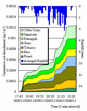
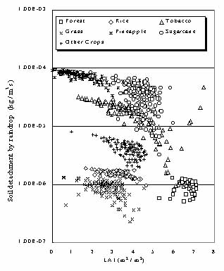
Fig. 1 In rainfall event 1,(a) cumulative soil detached per unit area; (b) soil detachment rate to increasing LAI for the same land use at maximum rainfall intensity.
The relative contribution of different vegetation types to the accumulated soil detached is shown in Fig. 1(a), with losses averaging 1.22 g m-2. This translates to about 14.1 tons of soil removed for the 5-hour, 36 mm rainfall. From Fig. 1 (b) it can be surmised that the detachment rate of soil due to raindrop impact either by leaf drip or direct rainfall is strongly influenced not only by the fraction of vegetation it encounters but also varies according to the type of vegetation involved and its abundance. It can also be deduced from Fig. 1(b) that the detachment mechanics can be confidently estimated from lesser LAI values and becomes more varied as vegetative cover thickens (i.e. high LAI).
The general trend that low LAI values lead to high soil detachment rates is observed. However, this was not the case for tobacco, pineapple and sugarcane crops, areas which, even with high abundance of leaf cover experience high detachment rates. In contrast, grass fields having lower LAI values yields lower detachment rates. Other surface conditions such as effects of tillage or absence thereof and other forms of disturbances on soil structure may be a plausible explanation for this observation and is subject for further investigation.
The condition for paddy rice fields however should be interpreted with care, since while the soil is open at the early stages of growth, as what is the existing condition at the time of the aerial photography, unlike other crops, it does not react directly with impacting rain by the ponded water which reduces sensitivity to DR. This may explain the almost level plot of detachment rate against increasing LAI.
3.2 Sediment discharge and turbidity plots
Table 1 presents a summary results of the comparison between observed simulated peak water discharge, sediment discharge and runoff for the four runoff events. Results of the sediment yield discharge modeling on four rainfall events are shown in Fig. 2, with the actual sediment discharge rates plotted from the turbidity sensor at the downstream portion of the river. For all the four rainfall events, the simulated sediment discharge peaks earlier than that measured by the turbidity sensor but all of them occur after the maximum water discharge.
| Peak water discharge (m3 s-1) | Delay in time to peak (min) | Peak sediment discharge m3 s-1 | Delay in time to peak (min) | Peak runoff (mm) | Delay in time to peak (min) | |||
| Obs. | Sim. | Obs. | Sim. | Obs. | Sim. | |||
| 62.24 | 74.56 | 7.833 | 658.92 | 668.49 | 16.6 | 2095 | 2105 | 7.33 |
| 46.25 | 54.03 | 4.666 | 651.114 | 562.34 | 13.3 | 1667 | 1707 | 5.00 |
| 21.06 | 26.36 | 3.5 | 552.296 | 535.58 | 21.5 | 1356 | 1393 | 2.833 |
| 54.64 | 60.77 | 5.33 | 680.025 | 953.65 | 3.43 | 1757 | 1802 | 5.17 |
Linear regression results report of R2 fits of 0.98, 0.67 and 0.97 between the observed versus the estimated peak runoff, water and sediment discharges respectively, almost all of which tend to match expected values but with discrepancies in timing. Although peak sediment discharge fits poorest, an examination of its time series plot in Fig. 2 suggests a realistic rendition of the sediment behavior in the channel flow. For an uncalibrated watershed, the results of the simulation already yield promising results to warrant further refinement of the input parameters. One data deficiency in the sediment yield model lies with the description of the initial bed conditions and the sediment sources along the channel. For example, the existence of grasses lying within the river beds may be responsible for the delay in discharge peaks but was not considered in the parameterization of channel flow.
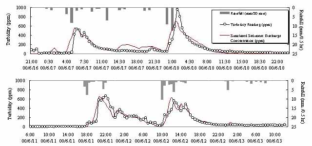
Fig. 2 Comparison of the simulated and measured sediment discharges for the 4 rainfall events.
4. Concluding Remarks
This paper presented an application of spectral unmixing technique to remotely-sensed data as an input to distributed sediment yield modeling with consideration for spatial variations in topographic, soil and vegetation cover conditions. It was observed that the rate of soil detachment varies with the type of vegetation cover and its abundance. The four rainfall events simulated show a satisfactory reproduction of the observed sediment discharge magnitudes but some discrepancy in the timing of the simulated discharge peak exists.
Future work should take into account the variation of vegetation growth conditions into the unmixing process. This requires acquisition of a time-series spectral signatures for the vegetation and soil cover. The sediment yield model should likewise be modified to incorporate the effects of physical characteristics of the channel bed. Coupled with these innovations, improved and integrated remote sensing and hydrologic methods can be attained and applied to monitor environmental degradation due to soil losses.
5. References
- Dikou, A., and T. Takeaki, 1999. Red-clay erosion in Okinawa Prefecture, Japan, Current status. Ambio, 28(6), pp. 534-535.
- Settle, J.J. and N.A. Drake, 1993. Linear mixing and the estimation of ground cover proportions. International Journal of Remote Sensing, 14(6), pp. 1159-1177.
- Gilabert, M. A., F.J. Garcia-Haro and J. Melia, 2000. A mixture modeling approach to estimate vegetation parameters in remote sensing. Remote Sensing of Environment,72(3), pp. 328-345.
- Wang, M., and A. Hjelmfelt, 1998. DEM-based overland flow routing model. Journal of Hydrologic Engineering, 3(1), pp. 1-8.
- Wicks, J.M. and J.C. Bathhurst, 1996. SHESED: a physically-based, distributed erosion sediment yield component for the SHE hydrological modeling system. Journal of Hydrology, 175, pp. 213-238.
- Van Leeuwen, W.J.D, A. R. Huete, C.L Walthall, S.D. Prince, A. Begue and J.L Roujean, 1997. Deconvolution of remotely sensed spectral mixtures for the retrieval of LAI, faPAR and soil brightness. Journal of Hydrology, 188-189, pp. 697-724.