| GISdevelopment.net ---> AARS ---> ACRS 2000 ---> SAR/InSAR |
Doppler Coefficient
Estimation for Synthetic Aperture Radar Using Sub-Aperture
Interferogram
Jim Min Kuo, K. S.
Chen
Institute of space Science, National Central University, Chung-Li, Taiwan
TEL:866-3-4227151 ext.7644; FAX: 866-2-22450943
E-mail: jmguo@mail2000.com.tw; mailto:dkschen@csr900.csrsr.ncu.edu.tw
Keywords
: Synthetic Aperture Radar, Sub-Aperture Interferogram, chirp
signalInstitute of space Science, National Central University, Chung-Li, Taiwan
TEL:866-3-4227151 ext.7644; FAX: 866-2-22450943
E-mail: jmguo@mail2000.com.tw; mailto:dkschen@csr900.csrsr.ncu.edu.tw
Abstract
A moving target will change the doppler coefficients of the received signal of Synthetic aperture radar(SAR), so we need to compute the coefficients, then we can obtain the moving targets speed or avoid smear of SAR images. This paper describes a new approach for estimating the doppler coefficients. Our approach uses the sub-aperture Interferogram scheme to estimate the doppler coefficients. Closed-form expressions are derived, and simulation results show this method can estimate the coefficients accurately. Less computation and a smaller amount samples of the signals are the characteristics of the Sub-Aperture Interferogram than other algorithms.
1. Introduction
Synthetic aperture radar (SAR) uses match filters to process the chirp signal to produce an accurate, high resolution images. A presence of moving targets, however, induces unwanted phase variations, resulting image degradations due to range migration. In addition, smeared and ill-positioned images with respect to the stationary background are caused as well. Hence, an estimate of the moving target relation to the antenna is necessary in order to improve the SAR images[1]. On the other hand, these estimates allows us to determine the moving targets velocity. The later is the purpose of this paper.
There are many works on how to estimate the phase coefficients. Based on the fact that the moving target and stationary background induce different doppler spectra, a detecting method was proposed in [2]. The method requires the use of a high pulse repetition frequency (prf) and performs poorly as the moving targets have a small range velocity components. Soumekh et al.[3] described the relation of the phase coefficients and the center frequency of doppler spectrum based on the short time Fourier transform (STFT). But as is well known, in STFT the resolution was limited either in time or in frequency domain, and it suffers from smearing and side-lobe leakage. Some methods use regression on the unwrapping signal phase [4] to estimate the polynomial phase coefficients of a constant amplitude signal, which requires to use a phase unwrapping algorithm prior to coefficient estimation. The algorithms is based on accumulate the phase difference, but it can be fooled by spare, rapidly changing phase values, and phase unwrapping errors cause inaccurate coefficient estimates. Another method by maximum likelihood estimation[5], it performs well at low SNR, but its cost is high computational complexity.
An estimation algorithm based on sub-aperture interferometric scheme and phase shift measurement to estimate the doppler coefficients is proposed in this paper. This paper also addresses the relation of target speed with the phase shift. Basically, the phase of the observed sequence is model as a polynomial embedded in white noise, which implies that, first, select an appropriate sub-aperture size and then segment recorded data to a finite number of subsets with the same size. Second, we can estimate the doppler parameters from the phase shift.
The presentation of the paper is as follows. First the problem of moving target velocity estimation in SAR signal is stated. Then a SAR signal model of a moving target velocity estimation is given in section II. Then a method for estimate doppler parameters is proposed in section III, which based on the application of interferometric scheme. And simulation results is shown in section IV. Finally, a conclusion is provided.
2. SAR Signal Model of A Moving Target
A moving target will alter the coefficients of the phase function of observed signals and target motion is generally unknown. When a conventional SAR processing algorithm is applied to scene with moving targets, the images of a moving targets are typically mislocated and smeared due to phase errors induced by the motion. The relation between antenna and a moving target can be express as a function of time and distance[1],[3]
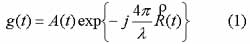
Where A(t) is the amplitude of the signal,
 is
the distance vector between target and antenna, and l is the wave length of SAR. This magnitude of will be denoted as ½½. For small time variations, ½½ is large relative to the magnitudes of the velocity
and acceleration vectors, and neglecting terms higher than t3
in a Taylor series expansion of the magnitude, then we can obtain the
expansion:
is
the distance vector between target and antenna, and l is the wave length of SAR. This magnitude of will be denoted as ½½. For small time variations, ½½ is large relative to the magnitudes of the velocity
and acceleration vectors, and neglecting terms higher than t3
in a Taylor series expansion of the magnitude, then we can obtain the
expansion: 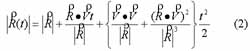
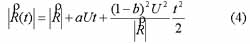
where V is the velocity contains both radar and moving target. We denote the moving target velocity vector as (vx,vy), which is the components of moving target velocity in range and azimuth respectively, and the along track's speed of the radar symbolized as U. The relation of moving speed to antenna speed can be expressed as:
Where (a,b) is the dimensionless of target's velocity scaled to the speed of the radar, and Normally, |a| and |b| <<1. From above mention we can assume that (a, b) is nearly constant during the integration time in the azimuth.
Using equation (2) and (3), (2) can be rewritten as follows:
Let Ut=y, the magnitude in (4) can be rewritten as followers:
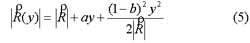
Using equation (1) and (5), the received signals can be written as:
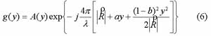
This is a signal of the linear FM form. Where A(y) will be considered a nuisance parameter and will not be estimated.
3. Estimation of the Chirp Signal Coefficient
From section II, we know SAR signal is a typical chirp signal and in general, is blurred by noise. We use a discrete-time polynomial phase signal model for the source signal, the measured data are assumed to consisted of signal and noise,

where y(y) is the phase of the signal, y0 is the initial point, T denote the total number of samples and r is sample spacing on the synthetic aperture of SAR, and n(y) denote multiply noise, it can be assumed as a zero mean white Gaussian noise[4,5,6]. The phase of the chirp signal is
where f0, f1, f2 are its initial phase, initial frequency and frequency rate, respectively. The principle value of the phase function of the measured signal can be expressed as
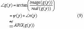
where -p<=Ðg(y)<=p, it can be computed from the data.
With the recorded data set of M elements, we generate a finite number of subsets with the same size N, what we call sub-apertures, by sequentially not overlapping each other.
SAj denote the j-th sub-aperture; and sub-aperture sizes is express as DY for convention, it is equal to samples N multiply sample spacing,DY=N*r . Based on the above-mentioned, the interferometric phase is come from (j+1)-th sub-aperture signal interfere with j-th sub-aperture signal, which is denote as fj(y) :
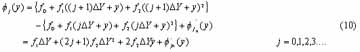
Where f¢jn(y) is the phase noise sequence and 0<y£N*r for a sub-aperture. Follow equation (10) we can obtain:

We use ERS SAR as the simulation system, to illustration it. We will assume that the electromagnetic behavior of the moving targets is similar to one point scatter response. The magnitude of the slant range is 8.4848e+005km, aircraft altitude is 800000m, azimuth sample spacing is 3.990574m and total samples is 1068, aircraft ground speed is 6.699028e+03m/sec, platform heading is 192.036610832947° and radar wavelength is 0.056666m, target heading is 161°, target speed is 9m/sec.
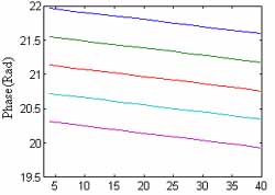
Some of the interferometric phase fj are shown in Figure 1. By this procedure the phase history from curve transform to linear and then the phase shift between fj+1(y) and fj(y) are constant. Compare equation (10) and (11), we can obtain the phase shift:
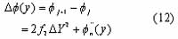
From equation (12) we can estimate a frequency rate f2i in every subsets of the measured signal:
Using equation (13) and after some manipulations, one can obtain the following estimate for the frequency rate
 :
:
Once
is available, then substitute it to the
below equation 
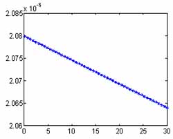
Follow the above-procedure of (10), we can obtain

Some of the interferometric phase
 are shown in
Figure.2. Compare equation (10) with (16), we know the phase difference
between and fj is
are shown in
Figure.2. Compare equation (10) with (16), we know the phase difference
between and fj is 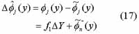
From the equation (17), we can estimate the value of the frequency fli:
The last result of
 is
is 
In the next section we show how to use this method for estimating a moving target speed in SAR.
4. Simulations
We use ERS SAR as the simulation system, the parameters were the same as previous case, except that moving target speed, target heading, and sub-aperture size.
For convenience, we reference equation (8) to rewritten (6) as a type chirp signal form
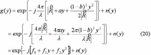
We assume that a moving target heading is 161°, moving speed vary from 0.1m/sec to 30m/sec and the sub-aperture size is 39.90574m. We can to estimate the coefficient of
and by follow the procedure of sub-aperture
interferometry method described in section III. The relational frequency
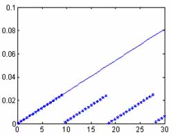
rate f2 and estimate result of is display in Figure.3, we can find the
estimate results agree very well with the truth coefficient. The frequency
f1 and estimated results ofis display in Figure.4. To observed the
variation of Figure.4, we find when that f1DY is larger than 2p thenis deviant. Which is caused by the
original signal is wrapped by 2p , and therefore
the limit of interferometric approach is that the absolute value of
2f2DY2 and
f1DY have to be smaller than 2p. In addition, we can obtain the minimum velocity of
moving targets is restricted within the resolution of phase of SAR.
In last, we summarize, the estimation procedure consists of six steps:
Step 1: Select a appropriate sub-aperture size and then segment recorded data to a finite number of subsets with the same size.
Step 2: transform {Ðg(y)} into {fj(y)} by equation (10).
Step 3: evaluate the phase difference by equation (12). Step 4: use equation (13) to estimate
;Step 5: Once
is available, follow equation (16) to
obtain {(y)} ; Step 6: evaluate the phase difference between{fj(y) and {
(y)} , to obtain ; 5. Conclusion
In this paper, we have developed an algorithm for estimate the coefficients of chirp signal. Through some analysis, we proved the relation of a phase difference of a series subsets' interferometric signals with the coefficients of chirp signal. In this algorithm, the coefficients
andare contrary to the sub-aperture size
DY . So sub-aperture sizes selection is a
trade-off between the target velocity and noise. We finally applied the algorithm to estimate the target speed of a simulation data of ERS SAR signals. Computer simulation results agree very well with the theoretical performance derived. And we find that the cost of computation is fewer and only need a small amount of samples of the data compare to some other methods.
Current, this algorithm is confined to use the principle value of the phase function, so to overcome this restriction, it could be to estimate the higher-speed's target and support a lower SNR of a signal.
Refferences
- J. Patrick Fitch, "Synthetic Aperture Radar," New York : Springer-Verlag , 1988.
- R.K. Raney, "Synthetic aperture imaging radar and moving target," IEEE Trans. Aerospace and Electronic Systems, Vol. AES-7, pp. 499-505, 1971.
- Soumekh Mehrdad, "Fourier array imaging," Englewood Cliffs, N.J : PTR Prentice-Hall, c1994.
- Slocumb, B.J.; Kitchen, J., "A polynomial phase parameter estimation-phase unwrapping algorithm," ICASSP-94: IEEE International Conference on Acoustics, Speech, and Signal Processing, vol. 4, pp. 129 -132, 1994.
- Besson, O.; Ghogho, N.; Swami, A., "Parameter estimation for random amplitude chirp signals ," IEEE Transactions on Signal Processing, vol. 47, pp 3208 -3219,1999.
- Jong-Sen Lee, Karl W. Hoppel, "Intensity and phase statistics of multilook polarimetric and interferometric SAR imagery", IEEE Transactions on Geoscience and Remote Sensing v 32 n 5 p 1017-1027, Sept 1994.
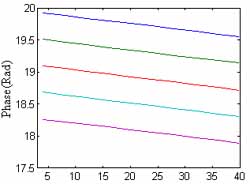 Azimuth position(meter) Figure.1. The histories of some interferometric signals phase from the original signal |
 Azimuth position(meter) Figure.2. The histories of some interferometric signals phase from the dechirped signal |
 Velocity(m/sec) Figure.3. The frequency rate f2 and estamate results . f2: solid line, " *
": |
 Velocity(m/sec) Figure.4. The frequency f1 and estimate result . f1: solid line, " *
":
|