| GISdevelopment.net ---> AARS ---> ACRS 2000 ---> Poster Session 3 |
Groundwater Prediction
Potential Zone in Langat Basin using the Integration of Remote Sensing and
GIS
1Khairul Anam
Musa, 2Juhari Mat Akhir and 2Ibrahim Abdullah
1Malaysian Centre for Remote Sensing (MACRES)
No.13, Jalan Tun Ismail, 50480 Kuala Lumpur
2Universiti Kebangsaan Malaysia, 43600 Bangi, Selangor Malaysia
1Malaysian Centre for Remote Sensing (MACRES)
No.13, Jalan Tun Ismail, 50480 Kuala Lumpur
2Universiti Kebangsaan Malaysia, 43600 Bangi, Selangor Malaysia
Abstract
Groundwater constitutes an important source of water supply for various purposes, such as domestic industries and agriculture needs. In the hydrological cycle, groundwater occurs when surface water (rainfall) seeps to a greater depth filling the spaces between particles of soil or sediment or the fractures within rock. Groundwater flows very slowly in the subsurface toward points of discharge, including wells, springs, rivers, lakes, and the ocean. In this study, the integration of remote sensing and geographic information system (GIS) method were used to produce map that classified the groundwater potential zone to either very high, high, moderate, low or very low in terms of groundwater yield. Almost all alluvial plains have a high potential of groundwater occurrence. Meanwhile, in the hard rock areas, groundwater potential is in the high density lineament zones.
1.0 Introduction
Groundwater forms the part of the natural water cycle, which is present within underground strata. The principle sources of groundwater recharge are precipitation and stream flow (influent seepage) and those of discharge include effluent seepage into the streams and lakes, springs, evaporation and pumping (Gupta, 1991). Ground water cannot be seen directly from the earth's surface, so a variety of techniques can provide information concerning its potential occurrence. Geological methods, involving interpretation of geologic data and field reconnaissance, represent an important first step in any ground water investigation. Remote sensing data from aircraft or satellite has become an increasing valuable tool for understanding subsurface water condition (Todd, 1980). They are particularly useful, very detailed and also show up features which cannot be seen easily on the ground. The various surfacial parameters prepared from remotely sensed data and ancillary data can be integrated and analyzed through GIS to predict the potential of ground water zone.
2.0 Objectives
The objectives of this study are as follows:
Langat Basin is located in south of Selangor and north of Negeri Sembilan within latitude 2°40'U to 3°20'U and longitude 101°10'E to 102°00'E with the geographical area extent of around 2,394.38 km2 (Figure 1).
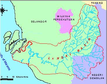
Figure 1: Map showung the location of the study area.
4.0 Methodology
In order to prepare the map showing potential zone for groundwater, five stages were applied; Source Data Collection, Image Processing, Building Database, Data Processing and Data Integration as outlined in Figure 2.
4.1 Source Data Collection
The Landsat TM data acquired on 6 March 1996 was collected together with the geological maps sheets 93, 94, 95, 101, 102 and 103 on 1:63,360 scale, prepared by the Minerals and Geoscience Department (JMG); topography maps sheets 3858, 3657, 3757, 3857, 3656, 3756, 3856, 3755 and 3855 on 1:50,000 scale, prepared by Survey and Mapping Department (JUPEM); rainfall data from 1982 to 1996 collected by the Meteorology Department of Malaysia, Drain and Drainage Department (JPS) and Universiti Kebangsaan Malaysia (UKM), soil series map of the study area on 1:150,000 scale, prepared by the Agriculture Department of Malaysia. In addition, hydrogeological map of Peninsular Malaysia on a scale of 1:500,000 and borehole data collected by the JMG were also utilized.
4.2 Satellite Data Analysis
The main task in this stage is to do an analysis and interpretation of satellite data, in order to produce basic maps such as structural and land use map in digital form. Basically, satellite data registration, correction and other image processing (such as enhancement, filtering, classification and other GIS process), together with field checking of the relevant area will be applied in this stage.
4.3 Spatial Database Building
The main task is to bring all the appropriate data (from stage 2 and existing relevant data) together into a GIS database. Basically, all the available spatial data will be assemble in the digital form, and properly registered to make sure the spatial component will overlap correctly. Digitizing of existing data and the relevant processing such as transformation and conversion between raster to vector, griding, buffer analysis, box calculating, interpolation and other format will also be conducted. This stage produces derived layers such as annual rainfall, lithology, lineament density, topography elevation, slope steepness, drainage density, land use and soil type.
4.4 Spatial Data Analysis.
This stage will process all the input layer from stage 2 and 3 in order to extract a spatial features which are relevant to the groundwater zone. This phase includes various analysis such as table analysis and classification, polygon classification and weight calculation. Polygons in each of the thematic layers were categorised depending on the recharge characteristics and suitable weightages were assigned (Table 1-8). The values of the weightage are based on Krishnamurthy et al. (1996 & 1997).
4.5 Data Integration
The final stage involves combining all thematic layers using the method that is modified from DRASTIC model, which is used to assess ground water pollution vulnerability by Environmental Protection Agency of the United State of America (Aller, 1985). The formula of the groundwater potential model (GP) as shown below:
GP = Rf + Lt + Ld + Lu + Te + Ss + Dd + St
where:
Rf:annual rainfall, Lt:lithology, Ld:lineament density, Lu:land use,
Te:topography elevation, Ss:slope steepness, Dd:drainage density and St:soil type.
The output is then reclassed into five groups such as very high, high, moderate, low and very low using the Quantile classification method (ESRI, 1996). The output that is produced is capable of being used for further investigations and assessments, especially at larger scale.
5.0 Result and Discussion
The ground water potential map of the Langat Basin area is shown in figure 3. In order to produce the map, a GIS model has been used, to integrate thematic maps such as annual rainfall, lithology, lineament density, land use, topography elevation, slope steepness, drainage density and soil type. Each thematic layer consists of a number of polygons, which correspond to different features. The polygons in each of the thematic layers have been categorized, depending on the suitability/relevance to the ground water potential, and suitable weights were assigned. Finally, all the thematic layers were integrated using the ground water potential model to derive the final derived layers. The score values of the area in the final map are shown Table 9.
Table 1 : Landuse
Table 2: Lineament Density
Table 3: Annual Rainfall.
Table 4 : Lithology.
Table 5 : Topography Elevation
Table 6 : Slope Steepness
Table 7 : Drainage Density
Table 8 : Soil Type
Table 9: Score values of the area polygons in the final map.
A summary of the results (Table 10), shows that almost all alluvial plains have high potential of groundwater occurrence. Where as, in steeply mountainous areas underlain by granite with low lineament density, the potential for groundwater is very low. Meanwhile in hard rock areas, the groundwater potential is high in areas with high lineament density and low drainage density.
Borehole data collected by the Minerals and Geoscience Department were used to compare the final results with the actual field data.
6.0 Conclusion
Based on this study, several conclusions can be made and they are:
The authors wish to thank Mr. Nik Nasruddin Mahmood (Director of MACRES), staff of MACRES and UKM for their comments and support in this project.
ReferencesTable 10: Summary of the results.
Note:
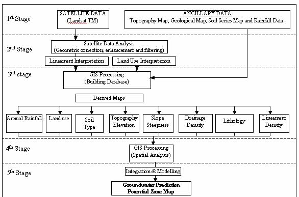
Figure 2: Methodology flowchart for groundwater potential zone mapping.
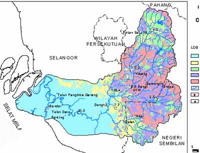
Figure 3: Groundwater potential map of the Langat Basin
Groundwater constitutes an important source of water supply for various purposes, such as domestic industries and agriculture needs. In the hydrological cycle, groundwater occurs when surface water (rainfall) seeps to a greater depth filling the spaces between particles of soil or sediment or the fractures within rock. Groundwater flows very slowly in the subsurface toward points of discharge, including wells, springs, rivers, lakes, and the ocean. In this study, the integration of remote sensing and geographic information system (GIS) method were used to produce map that classified the groundwater potential zone to either very high, high, moderate, low or very low in terms of groundwater yield. Almost all alluvial plains have a high potential of groundwater occurrence. Meanwhile, in the hard rock areas, groundwater potential is in the high density lineament zones.
1.0 Introduction
Groundwater forms the part of the natural water cycle, which is present within underground strata. The principle sources of groundwater recharge are precipitation and stream flow (influent seepage) and those of discharge include effluent seepage into the streams and lakes, springs, evaporation and pumping (Gupta, 1991). Ground water cannot be seen directly from the earth's surface, so a variety of techniques can provide information concerning its potential occurrence. Geological methods, involving interpretation of geologic data and field reconnaissance, represent an important first step in any ground water investigation. Remote sensing data from aircraft or satellite has become an increasing valuable tool for understanding subsurface water condition (Todd, 1980). They are particularly useful, very detailed and also show up features which cannot be seen easily on the ground. The various surfacial parameters prepared from remotely sensed data and ancillary data can be integrated and analyzed through GIS to predict the potential of ground water zone.
2.0 Objectives
The objectives of this study are as follows:
- To collect the ancillary data and to analyze the remote sensing data for getting information that is related to groundwater occurrence.
- To prepare difference thematic maps from the above information.
- To predict the groundwater potential zone through the various thematic maps using GIS technique.
- To develop a GIS model to identify groundwater potential zones.
- To show the integration of remote sensing and GIS techniques for prediction of the groundwater potential zone in the study area.
Langat Basin is located in south of Selangor and north of Negeri Sembilan within latitude 2°40'U to 3°20'U and longitude 101°10'E to 102°00'E with the geographical area extent of around 2,394.38 km2 (Figure 1).
Figure 1: Map showung the location of the study area.
4.0 Methodology
In order to prepare the map showing potential zone for groundwater, five stages were applied; Source Data Collection, Image Processing, Building Database, Data Processing and Data Integration as outlined in Figure 2.
4.1 Source Data Collection
The Landsat TM data acquired on 6 March 1996 was collected together with the geological maps sheets 93, 94, 95, 101, 102 and 103 on 1:63,360 scale, prepared by the Minerals and Geoscience Department (JMG); topography maps sheets 3858, 3657, 3757, 3857, 3656, 3756, 3856, 3755 and 3855 on 1:50,000 scale, prepared by Survey and Mapping Department (JUPEM); rainfall data from 1982 to 1996 collected by the Meteorology Department of Malaysia, Drain and Drainage Department (JPS) and Universiti Kebangsaan Malaysia (UKM), soil series map of the study area on 1:150,000 scale, prepared by the Agriculture Department of Malaysia. In addition, hydrogeological map of Peninsular Malaysia on a scale of 1:500,000 and borehole data collected by the JMG were also utilized.
4.2 Satellite Data Analysis
The main task in this stage is to do an analysis and interpretation of satellite data, in order to produce basic maps such as structural and land use map in digital form. Basically, satellite data registration, correction and other image processing (such as enhancement, filtering, classification and other GIS process), together with field checking of the relevant area will be applied in this stage.
4.3 Spatial Database Building
The main task is to bring all the appropriate data (from stage 2 and existing relevant data) together into a GIS database. Basically, all the available spatial data will be assemble in the digital form, and properly registered to make sure the spatial component will overlap correctly. Digitizing of existing data and the relevant processing such as transformation and conversion between raster to vector, griding, buffer analysis, box calculating, interpolation and other format will also be conducted. This stage produces derived layers such as annual rainfall, lithology, lineament density, topography elevation, slope steepness, drainage density, land use and soil type.
4.4 Spatial Data Analysis.
This stage will process all the input layer from stage 2 and 3 in order to extract a spatial features which are relevant to the groundwater zone. This phase includes various analysis such as table analysis and classification, polygon classification and weight calculation. Polygons in each of the thematic layers were categorised depending on the recharge characteristics and suitable weightages were assigned (Table 1-8). The values of the weightage are based on Krishnamurthy et al. (1996 & 1997).
4.5 Data Integration
The final stage involves combining all thematic layers using the method that is modified from DRASTIC model, which is used to assess ground water pollution vulnerability by Environmental Protection Agency of the United State of America (Aller, 1985). The formula of the groundwater potential model (GP) as shown below:
GP = Rf + Lt + Ld + Lu + Te + Ss + Dd + St
where:
Rf:annual rainfall, Lt:lithology, Ld:lineament density, Lu:land use,
Te:topography elevation, Ss:slope steepness, Dd:drainage density and St:soil type.
The output is then reclassed into five groups such as very high, high, moderate, low and very low using the Quantile classification method (ESRI, 1996). The output that is produced is capable of being used for further investigations and assessments, especially at larger scale.
5.0 Result and Discussion
The ground water potential map of the Langat Basin area is shown in figure 3. In order to produce the map, a GIS model has been used, to integrate thematic maps such as annual rainfall, lithology, lineament density, land use, topography elevation, slope steepness, drainage density and soil type. Each thematic layer consists of a number of polygons, which correspond to different features. The polygons in each of the thematic layers have been categorized, depending on the suitability/relevance to the ground water potential, and suitable weights were assigned. Finally, all the thematic layers were integrated using the ground water potential model to derive the final derived layers. The score values of the area in the final map are shown Table 9.
| Landuse | Weight |
| Forest | 20 |
| Agriculture | 40 |
| Scrub | 30 |
| Wetland | 50 |
| Urban | 10 |
| Cleared Land | 10 |
| Water Body | 60 |
Table 2: Lineament Density
| Lineament Density (km/km2) | Weight |
| > 0.0075 | 60 |
| 0.0055 - 0.0075 | 50 |
| 0.0035 - 0.0055 | 40 |
| 0.0015 - 0.0035 | 30 |
| < 0.0015 | 20 |
Table 3: Annual Rainfall.
| Annual Rainfall (mm) | Weight |
| 2500 - 2750 | 70 |
| 2250 - 2500 | 60 |
| 2000 - 2250 | 50 |
| 1750 - 2000 | 40 |
| 1500 - 1750 | 30 |
Table 4 : Lithology.
| Lithology | Weight |
| Alluvium | 70 |
| Limestone | 40 |
| Phylite-Schist-Quarzit | 20 |
| Quartz vein | 5 |
| Volcanic | 30 |
| Granite | 10 |
Table 5 : Topography Elevation
| Elevation (m) | Elevation Zone | Weight |
| < 20 | Almost Flat Topography | 50 |
| 20 - 100 | Undulating Rolling Hilly | 40 |
| 100 - 500 | Hilly Steeply Disserted | 35 |
| 500 - 1000 | Steeply Dissected Mountainous | 25 |
| > 1000 | Mountainous | 10 |
Table 6 : Slope Steepness
| % Slope | Slope Gradient | Slope Zone | Weight |
| 0 - 7 | 0° - 3° | Almost Flat Topography | 50 |
| 8 - 20 | 4° - 9° | Undulating Rolling Hilly | 40 |
| 21 - 55 | 10° - 24° | Hilly Steeply Disserted | 30 |
| 56 - 140 | 25° - 63° | Steeply Dissected Mountainous | 20 |
| > 140 | > 63° | Mountainous | 10 |
Table 7 : Drainage Density
| Drainage Density (km/km2) | Weight |
| > 0.0055 | 10 |
| 0.0040 - 0.0055 | 20 |
| 0.0025 - 0.0040 | 30 |
| 0.0010 - 0.0025 | 40 |
| < 0.0010 | 50 |
Table 8 : Soil Type
| Soil Series | Soil Type | Weight |
| Keranji | Clay | 10 |
| Melaka-Durian-Muncung | Gravel clay-silty clay-clay | 20 |
| Muncung-Seremban | Fine sandy clay | 20 |
| Prang | Clay | 10 |
| Regam-Jerangau | Coarse sandy clay-clay | 30 |
| Selangor-Kangkung | Clay | 10 |
| Serdang-Bugor-Muncung | Fine sandy clay loam-fine sandy clay-clay | 30 |
| Serdang-Kedah | Fine sandy clay loam | 30 |
| Urban Land | Sandy clay | 30 |
| Steep Land | Coarse sandy clay | 40 |
| Peat Land | Clay | 10 |
| Tanah Lombong | Sand | 50 |
| Telemung-Akob-Lanar Tempatan | Sandy loam-sandy clay | 30 |
Table 9: Score values of the area polygons in the final map.
| Score/value | Class of groundwater zone | Estimate of discharge rate |
| > 285 | Very High | > 22 m3/hour/well |
| 260 - 380 | High | 18 - 22 m3/hour/well |
| 245 - 255 | Moderate | 14 - 18 m3/hour/well |
| 230 - 240 | Low | 10 - 14 m3/hour/well |
| < 225 | Very Low | < 10 m3/hour/well |
A summary of the results (Table 10), shows that almost all alluvial plains have high potential of groundwater occurrence. Where as, in steeply mountainous areas underlain by granite with low lineament density, the potential for groundwater is very low. Meanwhile in hard rock areas, the groundwater potential is high in areas with high lineament density and low drainage density.
Borehole data collected by the Minerals and Geoscience Department were used to compare the final results with the actual field data.
6.0 Conclusion
Based on this study, several conclusions can be made and they are:
- The indicators of groundwater occurrences are related to the hydrological cycle and these are rainfall distribution, land use, soil types, lithology, geological structures, elevation, slope and drainage features of the area.
- Satellite data has been proven to be very informative and useful for surface study, especially in detecting a surface features and characteristics such as lineaments and land use.
- In order to predict the groundwater potential zones, different thematic maps have been prepared. These include annual rainfall distribution, land use, lithology, lineament density, topography elevation, slope steepness, drainage density and soil type.
- In subsurface study, remote sensing could be used more effectively if it is supported by the suitable GIS approach or techniques and good background knowledge of the related application.
- Integrated assessment of thematic maps using a model developed based on GIS techniques is the most suitable method for groundwater potential prediction zoning.
- The methods and results of this study were effective only for groundwater zone prediction in hard rock terrain, but was less effective in the alluvium environment.
The authors wish to thank Mr. Nik Nasruddin Mahmood (Director of MACRES), staff of MACRES and UKM for their comments and support in this project.
References
- Aller, L., Bennett, T., Lehr, J.H. & Petty, R.J. 1985. DRASTIC: A Standard System for Evaluating Ground Water Pollution Potential Using Hydrogeologic Settings. EPA/600/2-85/018, R.S. Kerr Environmental Research Laboratory, U.S. Environmental Protection Agency, Ada, Oklahoma.
- Bonham-Carter, Graeme. 1994. Geographic Information Systems For Geoscientist: Modelling with GIS. Canada: Pergamon.
- ESRI. 1996. ArcView GIS, The Geographic Information System for everyone: USA: Environmental Systems Research Institute.
- Gupta, Ravi P. 1991. Remote Sensing Geology. New York: Springer-Verlag Berlin Heidelburg.
- Krishnamurthy, J., Venkatesa Kumar, N., Jayaraman, V. & Manivel, M. 1996. An approach to demarcate ground water potential zones through remote sensing and a geographical information system. International Journal of Remote Sensing, 7, 1867-1884.
- Krishnamurthy, J., Arul Mani, M., Jayaraman, V. & Manivel, M. 1997. Selection of Sites for Artificial Recharge Towards Groundwater Development of Water Resource in India. Proceeding of the 18th Asian Conference on Remote Sensing, Kuala Lumpur. 20 - 24 Oktober.
- Todd, David K. 1980. Groundwater Hydrology. 2nd Edition. New York: John Wiley & Son.
- Van Zuidam, R.A. 1979. Terrain Analysis and Classification Using Aerial Photographs. ITC Textbook of Photo Interpretation Vol. VII.
| Layers\Potential Zone | Very High | High | Moderate | Low | Very Low |
| Rainfall (mm) | M/L | H | VH | M | M/L/VL |
| Landuse | Agriculture/Water body/Wetland | Agriculture/Water body/Scrub | Forest | Agriculture | Forest/Cleared land/Urban |
| Soil Type | Clay | Fine sandy clay loam/Fine sandy clay/Clay | Coarse sandy clay /Sandy loam/Sandy clay/Clay | Gravel clay/Coarse sandy clay/Silty clay/Clay | Coarse sandy clay |
| Lithology | Alluvium | Phylite-Schist-Quarzit | Phylite-Schist-Quarzit/ Granite | Granite | Granite |
| Lineament Density (km/km2) | NE | VH | M/H | VL | L |
| Elevation(m) | <20 | <20/20-100 | 20-100 | 20-100/100-500 | 100-500/>1000 |
| Slope (%) | 0-7/8-20 | 21-55 | 21-55/56-140 | 56-140 | >140 |
| Drainage Density (km/km2) | VL/L/M | VL/M | M/H | M/VH | L/M |
Note:
| Rainfall (mm) | Lineament Density (km/km2) | Drainage Density (km/km2) |
|
| VL (Very Low) | 1500-1750 | <0.0015 | <0.0010 |
| L (Low) | 1750-2000 | 0.0015-0.0035 | 0.0010-0.0025/ |
| M (Moderate) | 2000-2250 | 0.0035-0.0055 | 0.0025-0.0040 |
| H (High) | 2250-2500 | 0.0055-0.0075 | 0.0040-0.0055 |
| VH (Very High) | 2500-2700 | >0.0075 | >0.0055 |
| NE - No Effect |
Figure 2: Methodology flowchart for groundwater potential zone mapping.
Figure 3: Groundwater potential map of the Langat Basin