| GISdevelopment.net ---> AARS ---> ACRS 2000 ---> Image Processing |
An Efficient Artificial
Neural Network Training Method Through Induced Learning Retardation:
Inhibited Brain Learning
Joel C. Bandibas
(Research Center, Cavite State University, Philippines)
Research Fellow, Land Evaluation and Development Laboratory
NGRI, Senbonmatsu, Nishinasuno, Tochigi Prefecture, 329-2739 Japan
Tel. 0081-287-377246
Fax: 0081-287-366629
e-mail:bandibas@ngri.affrc.go.jp
Kazunori Kohyama
Head, Land Evaluation and Development Laboratory
NGRI, Senbonmatsu, Nishinasuno, Tochigi Prefecture, Japan
Email: kohyama@ngri.affrc.go.jp
Keywords: Artificial Neural Network Satellite Image Inhibited Brain Learning
Abstract
This study focuses on the development of a training scheme to make a large artificial neural network learn faster during training. This involves the identification of the few connection weights in the neural network that are too "greedy" to change during training. It is assumed that these few units "monopolize" the modeling of the information classes in satellite images. The hugely unequal participation of the neural network units during training is assumed to be the reason for the network's difficulty to learn. This study formulates a training scheme by which the changes of the connection weights of the most active units are temporarily inhibited when they reached a predetermined deviation limit. A set of connection weight deviation limit and maximum number of connection weights to be inhibited is formulated. The procedure induces a temporary retardation of the artificial neural network to learn. Through this, the most active units' "monopoly" in the modeling of the information classes is minimized giving the less active ones higher chances of participating in the modeling process. This results to faster training speed and a more accurate artificial neural network. The training procedure is termed inhibited brain learning.
The developed training method is tested using a Landsat TM data of the study site in Nishinasuno, Tochigi Prefecture, Japan with 7 land cover types. The results show that the developed training scheme is more than two times faster than the conventional training method. The fastest training speed obtained using the inhibited brain learning method is 2495 iterations. The conventional training method requires 8239 and 6495 iterations for the small and large artificial neural networks, respectively. Furthermore, the trained artificial neural network using the developed procedure is more accurate (90.5 %) compared to the accuracy of the small network (82.0%) and the large network (88.3%), both trained using the conventional method.
Introduction
The modeling of the human brain has always been motivated by its high performance in complex cognitive tasks like visual and auditory pattern recognition. One of the products of this effort is the development of artificial neural network (ANN) computing for satellite image classification, where training of the ANN is the core of the modeling process. Although ANN-based satellite image classification methods are more robust than conventional statistical approaches, difficulties in their use relate to their long training time (Kavzoglu and Mather, 1999). The process is computationally expensive making the use of ANN in remote sensing impractical.
The search for the ANN computing method that is both efficient and accurate has been the object of research of the practitioners of ANN computing. Previous research works primarily focused on the determination of the most appropriate ANN architecture and size that result to higher efficiency during training. Indeed, ANN efficiency is related to its architecture (Kanellopoulos and Wilkinson, 1997). However, designing the best ANN architecture and size that learns fast during training is a difficult balancing task. In general, large networks take longer time to learn than the smaller ones. Faster learning smaller networks might be able to generalize and accurate when processing smaller number of information classes in satellite images, but they are inaccurate for processing data with large number of training patterns (Kavzoglu and Mather, 1999). Furthermore, smaller networks are also inaccurate when the information classes involved have high intra-class spectral variability. On the other hand, slower learning large networks are very accurate to identify training data and are capable of processing large number of training patterns. They can also cope well with satellite images where the information classes are spectrally heterogeneous. However, they have poor generalization capability (Karnin, 1990) and are proven to be inaccurate during the actual classification.
The high intra-class spectral variability of information classes in satellite images is more of a rule than an exception. Consequently, the use of a relatively large ANN for satellite image classification can be advantageous if it can be made efficient during training and accurate during the actual classification. This study aims at making a large ANN learns faster during training and improves its capability to generalize. This study successfully formulates a training scheme by which the ANN is induced to learn faster. The procedure also enables the ANN to generalize better making it more accurate during the actual classification. The training scheme is termed inhibited brain learning (IBL).
Methods
Inhibited Brain Learning
IBL is a training scheme by which the change of values of the connection weights of the most active ANN units is temporarily inhibited during training. The development of IBL training scheme is based from following assumptions:
- In large networks, some connection weights are too "greedy" to change during training compared to the majority of the connections
- These few "greedy" units "monopolize" the modeling of the information classes in the training data.
- Temporarily inhibiting the changes of these "greedy" units during training will increase the participation of the less active units in the modeling of the information classes in the training data.
1. Identification of the "greedy" connection weights (most active units) during the initial stage of training.
2. Inhibit the change of the values of the active units during training through "clamping" when they reached a set deviation limit.
3. Releasing the "clamped" connection weights when their number reaches a set limit.
The "Clamp and Release" (CAR) Approach
CAR was implemented to minimize the "monopolistic" tendency of the most active connection weights of the ANN during training. To achieve this goal, the values of the connections of the most active units have to be inhibited (clamped) from changing after reaching a predetermined deviation limit. Once these values are clamped, the error can just be minimized through the changes of the values of the less active unclamped units. Obviously, the number of clamped connection weights increases as the training proceeds as more units will reach the deviation limit. Definitely, learning will be significantly retarded if majority of the units will already be clamped. A limit then has to be established as to how many connections are to be clamped. Once this limit is reached, clamping will be stopped and all the clamped connections will be released. Figure 1 shows an example of the clamping sequence of the ANN units connections during training.
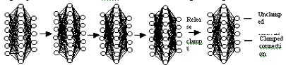 | |||||
| 0 iteration 0% clamped |
15 iteration 9.1% clamped |
26 iteration 16% clamped |
38 iteration 25% clamped |
38 iteration 0% clamped |
|
Figure 1. The clamp and release sequence during training of ANN with 25 percent clamped connection limit.
Connection Weights Deviation and Clamped Connections limits
CAR can just be implemented if the connection weights deviation and clamped connections limits are earlier determined. In this study, a series of experiments were conducted to determine the two important parameters to be used for the IBL. The values of the deviation limits used in this experiment, expressed in percent change of the initial values of the connection weights ranges from 25% to 300% at 25 % interval. On the other hand, the values of the clamped connection limits, expressed as percentage of the total number of connections of the ANN, ranges from 5% to 90% at 5% interval.
A Landsat TM data covering an area of 230 km2 was used for this experiment. The study area was located in Nishinasuno, Tochigi Prefecture, Japan. Training and test pixels were obtained through actual field visit of the study area. Seven land cover classes were considered in this study and they were the following: 1.) buildup areas; 2.) grassland; 3.) deciduous forest; 4.) coniferous forest; 5.) rice field; 6.) river and ; 7.) pond/dam.
Artificial Neural Network Structure
A multi-layer perceptron trained by the back-propagation algorithm (Rumelhart et al., 1986) using the gradient descent training method was used in this experiment. The ANN has one hidden layer with 30 nodes. The input layer has 5 nodes used to accommodate the 5 TM bands (bands 1 to 5) and the output layer consisted of 7 nodes reflecting the 7 land cover classes. For comparison purposes, two ANN of different sizes were trained using the conventional method and served as controls. The first ANN (control a) is a small network with 15 nodes in the middle layer and the second one (control b) has the same size as the networks trained using IBL. In this study, all ANN training were stopped after the trained networks reached an accuracy of at least 90% using the training data.
Results And Discussion
Training Speed
The results of the different training runs to determine the best combination of the deviation and clamped percentage limits that can give the fastest training time is shown in figure 2. Each line in figure 2 represents a deviation limit and shows the change in the number of iterations as the percentage of clamped connection increases. The two straight horizontal lines represent the number of iterations using the conventional training method (controls). It is very evident from the graph that most of the points are below the horizontal lines indicating that the IBL method results to faster training speed compared to the conventional one. Table 1 shows the fastest training speed of 2417 iterations (54.4 seconds) using the connection weight deviation and clamped connection limits of 225% and 15%, respectively. The conventional training method required 8239 iterations (101.6 seconds) and 6495 iterations (148.8 seconds) for the small ANN (Control a) and big ANN (Control b), respectively. The results also show that using the IBL, large ANN learn faster compared to the smaller ANN trained using the conventional method.
The effect of the clamped connection percentage is very evident in the experiment. The results show that training speeds were faster at clamped connection limits ranging from 15 to 45 percent. On the other hand, training speed did not significantly change when the clamped connection limits were 10 or lower at all levels of deviation limits. This indicates that only few active connections were identified at this level hence the effect on the training speed was minimal. On the other hand, training speed started to significantly decrease as the number of clamped connections goes beyond 85 percent. This result suggests that once the number of clamped connections reaches a critical mass, learning retardation will become very significant for only very few unclamped connections will be left to change to reduce the error.
The fastest training speeds were obtained at higher deviation limits and lower clamped connection limits. As indicated in figure 2, deviation limits ranging from 175 to 250 percent with clamped connection limits values ranging from 15 to 20 percent generated the best result. On the other hand, lower deviation limits generally yielded longer training time. This is because lower deviation limit will make connection weights that changes slightly qualify to be clamped. Consequently, more units will be clamped at the early stage of training which result to the significant retardation of the neural network to learn. On the other hand, higher deviation limits just allow connection weights that change significantly faster than most connection to be clamped. Because of this, the combination of higher deviation and lower clamped connection limits is sufficient to inhibit the changes of the "monopolistic" few connections in the ANN while giving more time for the less active units to participate in the error reduction process.
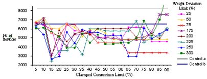
Figure 2. ANN training speed using different weight deviation and clamped connection limits values.
Accuracy
Artificial neural network accuracy is always related to its ability to generalize. Generalization is the ability of the neural network to interpolate and extrapolate data that it has not seen before (Atkinson and Tatnall, 1997). One of the most important factors that effect the ANN generalization capability is training time. The longer a network is trained the better it classifies the training data, but the more likely it is to fail in the classification of new data because it may become over-specific (Kavzoglu and Mather, 1999). In this study, the combination of deviation limits and clamped percentage limits that resulted to the shortest training time were determined. The accuracy of the trained networks obtained from these limit settings were investigated whether the shortened training time also resulted to the improvement of the network's ability to generalize.
Table 1 shows the combination of deviation and clamped connection limits that resulted to the fastest training speeds in the experiment. The training speeds and accuracy obtained using the conventional training method are also included for comparison. The results show that IBL method with deviation limits ranging from 175 to 250 percent with 15 % clamped percentage limit resulted to training speeds more than twice as fast as the controls. It also shows that using the IBL, the ANN's accuracy to identify test pixels is greater than those trained using the conventional method. These results indicate that with shortened training time, the ability of the ANN to generalize also improves. Furthermore, the large ANN trained using the IBL can generalize better than the small ANN trained using the conventional method. Figure 3 shows two classified images using trained ANN employing the conventional and the IBL training methods.
| Weight Deviation Limit (%) | Clamped Connection Limit (%) | Number of iterations | Training Time (seconds) | Accuracy (%) |
| control a (small ANN) | control a | 8239 | 101.6 | 82.0 |
| control b | control b | 6495 | 148.8 | 88.3 |
| 175 | 15 | 3135 | 75.5 | 89.1 |
| 200 | 15 | 2893 | 66.1 | 89.4 |
| 225 | 15 | 2417 | 54.4 | 90.0 |
| 250 | 15 | 2670 | 59.9 | 89.4 |
Conclusions
The inhibited brain learning training method proved to be a very simple, effective and promising procedure for training artificial neural network. The procedure significantly increased the training speed of a large network. Furthermore, the tendency of a large artificial neural network to be over specific, hence have less generalizing capability, was avoided through reduced training time. The procedure generated a trained large network that can generalize and more accurate for satellite image classification.
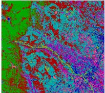 (a) |
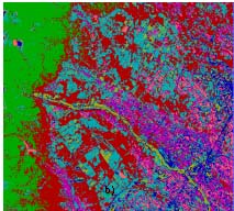 (b) |
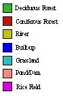 |
Figure 3. Classified satellite image using the trained ANN. Image a was generated using conventinal training ANN method (control b) and image b using with 225% deviation and 15% clamped connection limits, respectively.
References
- Atkinson, P.M., and Tatnall, A.R.L., 1997. Neural networks in remote sensing, International Journal of Remote Sensing, 18 (4), pp. 699-709.
- Kanellopoulos, I., and Wilkinson, G.G., 1997. Strategies and best practice for neural network image classification, International Journal of Remote Sensing, 18 (4), pp. 711-725.
- Karnin, E.D., 1990. A simple procedure for pruning back-propagation trained neural networks, IEEE Transactions on Neural Networks, 1, pp. 239-242.
- Kavsoglu, T., and Mather, P.M., 1999. Pruning artificial neural networks: an example using land cover classification of multi-sensor images, International Journal of Remote Sensing, 20 (14), pp. 2787-2803.
- Rumelhart, D.E., Hinton,G.E., and Williams, R.J., 1986. Learning internal representations by error propagation. In: Parallel Distributed Processing: Explorations in the Microstructure of Cognition, Volume 1: Foundations, edited by Rumelhart, D.E., McLelland, J.L., and the PDP Research Group (Cambridge, Massachusetts: MIT Press), pp. 318-362.