| GISdevelopment.net ---> AARS ---> ACRS 2000 ---> Image Processing |
A Synergistic Automatic
Clustering Technique (Syneract) for Multispectral Image Analysis
Kai-Yi Huang
Associate Professor, Department of Forestry,
National Chung-Hsing University,
250 Kuo-Kuang Road, Taichung, Taiwan 402
Tel: +886-4-2854663; Fax: +886-4-2873628
E-mail:kyhuang@dragon.nchu.edu.tw
Kai-Yi Huang
Associate Professor, Department of Forestry,
National Chung-Hsing University,
250 Kuo-Kuang Road, Taichung, Taiwan 402
Tel: +886-4-2854663; Fax: +886-4-2873628
E-mail:kyhuang@dragon.nchu.edu.tw
Keywords: Remote Sensing, Clustering Algorithm,
Unsupervised Classification
Abstract
ISODATA has been widely used in unsupervised and supervised classification. However, it requires the analyst to have a priori knowledge about the data for specifying input parameters. The beginner will spend much time on determining those parameters by trial and error. It is time-consuming because of its iterative process. The study aimed to develop a synergistic automatic clustering technique (SYNERACT) that combined the hierarchical descending and K-means clustering procedures to avoid limitations with ISODATA. They were compared according to classification accuracy and efficiency using two-date video images. An inappropriate seed assignment for ISODATA was shown to significantly reduce accuracies. In contrast, SYNERACT was required to specify only two parameters. It determined the locations of the initial clusters automatically from the data, thereby avoiding those limitations. Because SYNERACT passed through the data set in times largely fewer than ISODATA did, SYNERACT was much faster than ISODATA. SYNERACT also matched ISODATA in accuracy. Accordingly, SYNERACT was a suitable alternative for ISODATA in the multispectral image analysis.
1. Introduction
Multispectral image classification is one of the most often used techniques for extracting information from remotely sensed data of the Earth, which can be performed by unsupervised classification using clustering (Jensen, 1996). Clustering performs the valuable function of identifying some of the unique classes but with very small areal extent that might not be initially apparent to the analyst applying a supervised classifier. Therefore, the clustering method seems to be a much more practical approach for information extraction (Viovy, 2000). There are two main families of clustering methods: the Iterative Self-Organizing Data Analysis Techniques (ISODATA) clustering and hierarchical clustering approaches (Viovy, 2000).
The ISODATA (or K-means) algorithm is a widely used clustering method to partition the image data in the multispectral space into a number of spectral classes (Jensen, 1996). This type of clustering algorithms, however, suffers from several limitations. One of the limitations is that ISODATA requires the user to specify the number of clusters beforehand. The second limitation is that it requires the user to specify the starting positions of these clusters through an educated guess. The clustering starts with a set of arbitrarily selected pixels as cluster centers with exception no two may be the same (Swain, 1978). The choice of the initial locations of the cluster centers is not critical, but it will evidently affect the time it takes to reach a final, acceptable result (Richards, 1993). It does not matter where the initial cluster centers are located, as long as enough number of iterations is allowed (ERDAS, 1997). Because no guidance is available in general, a logical procedure is adopted in LARSYS (Richards, 1993). The initial cluster centers are chosen evenly distributed along the diagonal axis in the multidimensional feature space. This is a line from the origin to the point corresponding to the maximum digital number in each spectral component. Other similar procedures used in ISODATA have been proposed in Jensen (1996) and ERDAS (1997). However, few studies have investigated the problem for the past years about how random choice of the initial cluster centers and those procedures proposed by ERDAS (1997) and Jensen (1996) may affect final classification results. The study thus will examine this very important but apparently neglected problem.
The third limitation associated with ISODATA is its processing speed. ISODATA is computationally intensive when processing large data sets since, at each iterative step, all pixels in the whole data set must be checked against every cluster center. Furthermore, this method tends to suffer from performance degradation as the number of bands, the number of pixels, or the number of clusters increases (Richards, 1993; Viovy, 2000).
The second type of clustering methods that does not require the analyst to specify the number of clusters beforehand is hierarchical clustering (Richards, 1993). As pointed out by Richards (1993), a divisive hierarchical clustering (or hierarchical descending) algorithm has been developed in which the data are initialized as a single cluster that is progressively subdivided. This method is more computationally intensive and is rarely used in remote sensing image analysis since usually a large number of pixels are involved.
The goal of this study was to develop a synergistic automatic clustering technique (SYNERACT) that combined both hierarchical descending and K-means approaches to avoid before-mentioned limitations associated with ISODATA. The study attempted to accomplish the three specific objectives using two-date video image data. The first objective was to develop SYNERACT based on hyperplane, dynamical (iterative optimization) clustering principles, and binary tree. The second one was to compare SYNERACT with ISODATA in terms of classification accuracy and efficiency. The third one was to show that SYNERACT was very fast and well suited to act as a substitute for ISODATA in remote sensing applications, which was opposite to the ideas suggested by Richards (1993).
2. Study Area And Materials
The study area was located near Weslaco in Hidalgo county, Texas. It was a completely randomized block designed field experiment consisting of plots of the following surface features: (1) cotton, (2) cantaloupe, (3) sorghum, (4) johnsongrass, (5) pigweed, and (6) bare soil (Figure 1). Each of the 24 plots (six treatments and four replications) measured 7.11 m by 9.14 m, making the total site dimension 42.67 m by 36.56 m (Richardson et al., 1985). However, the fourth row (drawn with dash line) was excluded from the study due to damage of this portion of the video data file.
The two-date video image data were acquired on 31 May and 24 July 1983 near noon on moderately sunny days from an altitude of 900 m. The video imaging system used to collect data for the study is described in detail in Richardson et al. (1985). Spectral bands 1-4 were acquired on 24 July; spectral bands 5-8 were acquired on 31 May. Channels 1 and 5 were blue bands (420 to 430 nm), Channels 2 and 6 were red bands (640 to 670 nm), channels 3 and 7 were yellow-green bands (520 to 550 nm), and channels 4 and 8 were near-infrared bands (850 to 890 nm). Multiple-date image normalization using regression (Jensen, 1996) was performed to radiometrically correct the data set used in the study since atmospheric effects probably affected pixel brightness values of the two-date video image data. Accuracy assessment was performed over 18 plots from row 1 to row 3 in the experimental field with the exception of row 4.
3. Method and Rationale
SYNERACT in fact combines the concepts of hyperplane, iterative optimization clustering and binary tree. The hyperplane divides a cluster into two clusters of smaller size and computes their means. The iterative optimization clustering procedure (IOCP) is based on estimating some reasonable assignment of the pixel vectors into candidate clusters and moving them from one cluster to another in such a way that an objective function is minimized (Richards, 1993). The binary tree is a useful data structure that can store the clusters successively generated from each split. SYNERACT treats all of the image pixels as a single cluster. The single cluster is placed at the root of a binary tree firstly, and then is progressively subdivided. At each split, the algorithm will attempt to divide each cluster defined at the previous split into two clusters of smaller size and to compute their centers. IOCP is then performed. Each split is tested for relevance a posteriori. Two clusters of smaller size generated from each split by a hyperplane are placed at the left and right subtree nodes, respectively. If the test fails, the cluster will no longer be split in further separation. The cluster is called stabilized. This process continues until all clusters are stabilized.
3.1 Definition of a Hyperplane
To appreciate the development of SYNERACT, it is required to understand the concept of hyperplane. The family of linear discriminant functions (Nilsson, 1965) can be expressed in the form as follows:
f (X) = W1 * X1 + W2 *
X2 + . . . + Wn * Xn + Wn+1,
(1)
where W1, W2, . . . , Wn, Wn+1 are weighting coefficients. f is a linear function of the components of an augmented column vector X.
A simple linear separation is performed by a linear discriminant function that partitions the feature space into two regions. The linear discriminant function can be viewed as a separating surface in which the simplest form is a hyperplane (Nilsson, 1965). A hyperplane partitions the feature space into two regions defined as:
f (X) = W·X > 0 and f (X) = W·X
£ 0, (2)
where W = [W1, W2, . . . , Wn, Wn+1], Xt = [X1, X2, . . . , Xn, 1], and n = dimension of the feature space.
Assume that there is a cluster in the feature space. A weight vector W is viewed to implement a linear separating surface (hyperplane) to divide a cluster in the feature space into two clusters of smaller size (children). The augmented pixel vectors of the one child-cluster have a positive dot product value with W, while the other child-cluster consists of pixels (lying on the other side of W) that have a zero or negative dot product value with W. The former is categorized as S1 and the latter is categorized as S2. Centers of the two sets are computed according to all of the pixels in the two sets, respectively. The sets of parent cluster (S) and two child-clusters (S1and S2) can be defined as:
S1 = {XeS| W·X > 0};
S2 = {Xe S| W·X£0}; S = S1 È
S2.
3.2 Generation of a Hyperplane
An augmented pixel vector is defined as:
X = [Vt, 1]t , where Vt =
[V1,V2, . . . , Vn].
(3)
The process of generating a weight vector is illustrated in Figure 2. Let the pixels be augmented and expressed by the general column vector X. One pixel P is chosen from this cluster so that |P - C| > |X - C| for all X, where C is an arbitrarily chosen position vector in the feature space. Let C be the grand mean vector computed from all of the pixels in a single cluster. Under this condition, P and C define a line from the grand mean C to the farthest pixel P. Assume that there is a single cluster in the two-dimensional feature space consisting of two spectrally distinct clusters of smaller size represented by U and V, respectively so that {X} = {U} È {V}, Pe{X}. Assume further that P comes from {U} and is denoted by U*, U* = P. The next step is to find all of V so that (V - C)·(U* - C) £ 0 , {V} ( {X}. Find V1* or V2* from {V} so that V1* must satisfy |(V1* - C)·(U* - C)| = 0 and V2* must satisfy |(V2* - C)·(U* - C)| < |(V - C)·(U* - C)|. Since the brightness value of each pixel in remotely sensed data is recorded as an integer, V1* cannot always be found in all cases. Thus V2* having the biggest negative dot product value is used as an alternative of V1*. Lines perpendicular to (U* - C) and passing through V1* or V2* will be hyperplanes (weight vectors) separating {U} and {V}, as shown in Figure 2. According to the concept of the single-sided decision surface proposed by Lee and Richards (1984), these two hyperplanes (weight vectors) are defined by equations shown as follows:
W1 = [(U* - C)t , V1*·(U* - C) ]t
(4)
W2 = [(U* - C)t , V2*·(U* - C) ]t (5)
3.3 Test for Relevance of Splitting
SYNERACT will split each cluster formed at the previous separation into two clusters of smaller size. The splitting process is theoretically continued until there is only one pixel in each cluster. Therefore, this process must be controlled by two input parameters, including the maximum number of clusters to be considered (Cmax) and the minimum percentage of pixels allowed in a single cluster (P%). Each split is tested for these two parameters a posteriori in order that a homogeneous cluster will not be split inappropriately. Since each cluster is the basis for an information class, Cmax will become the maximum number of classes to be formed. Some clusters with number of pixels less than P% can be eliminated, leaving less than Cmax clusters. The pixels in these discarded clusters will be reassigned to an alternative cluster.
4. Results and Discussion
The two-date video image data used for testing two clustering algorithms had eight bands mentioned in section 2. The total number of band combinations (i.e. 8C8 +, . . . , + 8C1) was equal to 255. The band combination of 2, 3, 4, and 8 with best separability was chosen for the test using the program module Separability \ Euclidean Distance Measure in ERDAS Imagine 8.3.1 software.
4.1 Influences of Initial Seed Assignment
Table 1 presents the classification results of ISODATA using six sets of initial cluster centers randomly generated. Overall accuracies varied from the lowest 65% to the highest 85% for six sets of initial seeds randomly generated. Clearly, the choice of the initial locations of the cluster centers was critical, because it evidently affected final classification results. This outcome was contrary to the ideas proposed by Richards (1993) and ERDAS (1997).
This study also applied the procedure of initial seed assignment proposed by Jensen (1996) and ERDAS (1997) to specify the initial locations of the cluster centers required by ISODATA. Table 1 also presents the classification results generated from ISODATA using five initial seed allocations. In this case, µ±1*s had the best overall accuracy (93%) and µ±5*s had the lowest overall accuracy (75%), where µ is the mean vector and s is standard deviation; however, the analyst would have to spend much of his time on 'try and see' to determine an optimal number of standard deviations for other cases.
4.2 Efficiency
4.2.1 Processing Speed
Table 2 presents the lengths of computational time of two clustering algorithms varied with the number of pixels in the data set they processed and the number of clusters generated. The lengths of computational time spent by ISODATA were 6-39 (TI/TS) times as long as those spent by SYNERACT, as the number of pixels increased from 3,400 to 17,640 and the number of clusters was set 16. Table 3 presents the lengths of computational time of two clustering algorithms varied with different band combinations. The lengths of computational time spent by ISODATA were 6-12 (TI/TS) times as long as those spent by SYNERACT, as the number of bands varied between two and eight.
4.2.2 Ease of Use
A sophisticated ISODATA algorithm described by Jensen (1996) normally requires the analyst to specify seven parameters. The ISODATA program of ERDAS Imagine software requires the user to specify four parameters identical to some of parameters proposed by Jensen and to initialize cluster means along a diagonal axis or principal axis, but skips splitting and merging parameters. In contrast, SYNERACT developed in the study required the analyst to specify only two parameters already mentioned in section 3. Moreover, it eliminated the need for a priori estimates on the locations of the initial clusters. Accordingly, SYNERACT was more users-friendly for the beginner than ISODATA.
4.3 Classification Accuracy
Table 4 presents the overall accuracies and the accuracies of individual categories of the two clustering approaches. The overall accuracy (92%) of SYNERACT was only about 1% lower than that of ISODATA (93%); this difference was probably due to chance. Accordingly, SYNERACT and ISODATA were equally matched in classification accuracy.
5. Conclusions
SYNERACT required a minimum of user input with only two parameters, thereby reducing the load of specifying other complex parameters by trial and error on the beginner. By comparison, ISODATA was not users-friendly since it required the analyst to specify many input parameters, particularly the starting positions of the initial clusters. This study showed that an inappropriate choice of this parameter for ISODATA significantly reduced final classification accuracies. This outcome obviously was opposite to the ideas stated by Richards (1993) and ERDAS (1997). In contrast, SYNERACT had the ability to determine this parameter automatically from the data set itself, and thus avoided the adverse effect on a final clustering. SYNERACT was very fast, whereas ISODATA was time-consuming. SYNERACT had the capability to compete with ISODATA in classification accuracy. In sum, this study showed that SYNERACT was really efficient and well suited to serve as an alternative of ISODATA for applications in remote sensing image analysis involving a large data set, which was opposite to the thoughts proposed by Richards (1993).
References
Table 1. Classification Accuracies of
ISODATA Using Six Sets of Randomly Generated Initial Seeds and five sets
of ERDAS's Initial Seed Assignment.
Table 3. The Lengths of Processing Time Spent by SYNERACT and ISODATA for Seven Sets of Band Combinations.
Table 4. Classification Accuracies of the SYNERACT and ISODATA Methods.
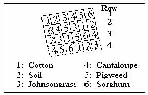
Figure 1. Plot Identification Map of the Study Area
(Not Drawn on the Scale).
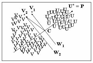
Figure 2. A Two-dimensional, Hypothetical Case with Two Clusters Illustrates the Process of Generating the Weight Vector W1 or W2 that Implements a Hyperplane of Hierarchical Descending Clustering.
Abstract
ISODATA has been widely used in unsupervised and supervised classification. However, it requires the analyst to have a priori knowledge about the data for specifying input parameters. The beginner will spend much time on determining those parameters by trial and error. It is time-consuming because of its iterative process. The study aimed to develop a synergistic automatic clustering technique (SYNERACT) that combined the hierarchical descending and K-means clustering procedures to avoid limitations with ISODATA. They were compared according to classification accuracy and efficiency using two-date video images. An inappropriate seed assignment for ISODATA was shown to significantly reduce accuracies. In contrast, SYNERACT was required to specify only two parameters. It determined the locations of the initial clusters automatically from the data, thereby avoiding those limitations. Because SYNERACT passed through the data set in times largely fewer than ISODATA did, SYNERACT was much faster than ISODATA. SYNERACT also matched ISODATA in accuracy. Accordingly, SYNERACT was a suitable alternative for ISODATA in the multispectral image analysis.
1. Introduction
Multispectral image classification is one of the most often used techniques for extracting information from remotely sensed data of the Earth, which can be performed by unsupervised classification using clustering (Jensen, 1996). Clustering performs the valuable function of identifying some of the unique classes but with very small areal extent that might not be initially apparent to the analyst applying a supervised classifier. Therefore, the clustering method seems to be a much more practical approach for information extraction (Viovy, 2000). There are two main families of clustering methods: the Iterative Self-Organizing Data Analysis Techniques (ISODATA) clustering and hierarchical clustering approaches (Viovy, 2000).
The ISODATA (or K-means) algorithm is a widely used clustering method to partition the image data in the multispectral space into a number of spectral classes (Jensen, 1996). This type of clustering algorithms, however, suffers from several limitations. One of the limitations is that ISODATA requires the user to specify the number of clusters beforehand. The second limitation is that it requires the user to specify the starting positions of these clusters through an educated guess. The clustering starts with a set of arbitrarily selected pixels as cluster centers with exception no two may be the same (Swain, 1978). The choice of the initial locations of the cluster centers is not critical, but it will evidently affect the time it takes to reach a final, acceptable result (Richards, 1993). It does not matter where the initial cluster centers are located, as long as enough number of iterations is allowed (ERDAS, 1997). Because no guidance is available in general, a logical procedure is adopted in LARSYS (Richards, 1993). The initial cluster centers are chosen evenly distributed along the diagonal axis in the multidimensional feature space. This is a line from the origin to the point corresponding to the maximum digital number in each spectral component. Other similar procedures used in ISODATA have been proposed in Jensen (1996) and ERDAS (1997). However, few studies have investigated the problem for the past years about how random choice of the initial cluster centers and those procedures proposed by ERDAS (1997) and Jensen (1996) may affect final classification results. The study thus will examine this very important but apparently neglected problem.
The third limitation associated with ISODATA is its processing speed. ISODATA is computationally intensive when processing large data sets since, at each iterative step, all pixels in the whole data set must be checked against every cluster center. Furthermore, this method tends to suffer from performance degradation as the number of bands, the number of pixels, or the number of clusters increases (Richards, 1993; Viovy, 2000).
The second type of clustering methods that does not require the analyst to specify the number of clusters beforehand is hierarchical clustering (Richards, 1993). As pointed out by Richards (1993), a divisive hierarchical clustering (or hierarchical descending) algorithm has been developed in which the data are initialized as a single cluster that is progressively subdivided. This method is more computationally intensive and is rarely used in remote sensing image analysis since usually a large number of pixels are involved.
The goal of this study was to develop a synergistic automatic clustering technique (SYNERACT) that combined both hierarchical descending and K-means approaches to avoid before-mentioned limitations associated with ISODATA. The study attempted to accomplish the three specific objectives using two-date video image data. The first objective was to develop SYNERACT based on hyperplane, dynamical (iterative optimization) clustering principles, and binary tree. The second one was to compare SYNERACT with ISODATA in terms of classification accuracy and efficiency. The third one was to show that SYNERACT was very fast and well suited to act as a substitute for ISODATA in remote sensing applications, which was opposite to the ideas suggested by Richards (1993).
2. Study Area And Materials
The study area was located near Weslaco in Hidalgo county, Texas. It was a completely randomized block designed field experiment consisting of plots of the following surface features: (1) cotton, (2) cantaloupe, (3) sorghum, (4) johnsongrass, (5) pigweed, and (6) bare soil (Figure 1). Each of the 24 plots (six treatments and four replications) measured 7.11 m by 9.14 m, making the total site dimension 42.67 m by 36.56 m (Richardson et al., 1985). However, the fourth row (drawn with dash line) was excluded from the study due to damage of this portion of the video data file.
The two-date video image data were acquired on 31 May and 24 July 1983 near noon on moderately sunny days from an altitude of 900 m. The video imaging system used to collect data for the study is described in detail in Richardson et al. (1985). Spectral bands 1-4 were acquired on 24 July; spectral bands 5-8 were acquired on 31 May. Channels 1 and 5 were blue bands (420 to 430 nm), Channels 2 and 6 were red bands (640 to 670 nm), channels 3 and 7 were yellow-green bands (520 to 550 nm), and channels 4 and 8 were near-infrared bands (850 to 890 nm). Multiple-date image normalization using regression (Jensen, 1996) was performed to radiometrically correct the data set used in the study since atmospheric effects probably affected pixel brightness values of the two-date video image data. Accuracy assessment was performed over 18 plots from row 1 to row 3 in the experimental field with the exception of row 4.
3. Method and Rationale
SYNERACT in fact combines the concepts of hyperplane, iterative optimization clustering and binary tree. The hyperplane divides a cluster into two clusters of smaller size and computes their means. The iterative optimization clustering procedure (IOCP) is based on estimating some reasonable assignment of the pixel vectors into candidate clusters and moving them from one cluster to another in such a way that an objective function is minimized (Richards, 1993). The binary tree is a useful data structure that can store the clusters successively generated from each split. SYNERACT treats all of the image pixels as a single cluster. The single cluster is placed at the root of a binary tree firstly, and then is progressively subdivided. At each split, the algorithm will attempt to divide each cluster defined at the previous split into two clusters of smaller size and to compute their centers. IOCP is then performed. Each split is tested for relevance a posteriori. Two clusters of smaller size generated from each split by a hyperplane are placed at the left and right subtree nodes, respectively. If the test fails, the cluster will no longer be split in further separation. The cluster is called stabilized. This process continues until all clusters are stabilized.
3.1 Definition of a Hyperplane
To appreciate the development of SYNERACT, it is required to understand the concept of hyperplane. The family of linear discriminant functions (Nilsson, 1965) can be expressed in the form as follows:
where W1, W2, . . . , Wn, Wn+1 are weighting coefficients. f is a linear function of the components of an augmented column vector X.
A simple linear separation is performed by a linear discriminant function that partitions the feature space into two regions. The linear discriminant function can be viewed as a separating surface in which the simplest form is a hyperplane (Nilsson, 1965). A hyperplane partitions the feature space into two regions defined as:
where W = [W1, W2, . . . , Wn, Wn+1], Xt = [X1, X2, . . . , Xn, 1], and n = dimension of the feature space.
Assume that there is a cluster in the feature space. A weight vector W is viewed to implement a linear separating surface (hyperplane) to divide a cluster in the feature space into two clusters of smaller size (children). The augmented pixel vectors of the one child-cluster have a positive dot product value with W, while the other child-cluster consists of pixels (lying on the other side of W) that have a zero or negative dot product value with W. The former is categorized as S1 and the latter is categorized as S2. Centers of the two sets are computed according to all of the pixels in the two sets, respectively. The sets of parent cluster (S) and two child-clusters (S1and S2) can be defined as:
3.2 Generation of a Hyperplane
An augmented pixel vector is defined as:
The process of generating a weight vector is illustrated in Figure 2. Let the pixels be augmented and expressed by the general column vector X. One pixel P is chosen from this cluster so that |P - C| > |X - C| for all X, where C is an arbitrarily chosen position vector in the feature space. Let C be the grand mean vector computed from all of the pixels in a single cluster. Under this condition, P and C define a line from the grand mean C to the farthest pixel P. Assume that there is a single cluster in the two-dimensional feature space consisting of two spectrally distinct clusters of smaller size represented by U and V, respectively so that {X} = {U} È {V}, Pe{X}. Assume further that P comes from {U} and is denoted by U*, U* = P. The next step is to find all of V so that (V - C)·(U* - C) £ 0 , {V} ( {X}. Find V1* or V2* from {V} so that V1* must satisfy |(V1* - C)·(U* - C)| = 0 and V2* must satisfy |(V2* - C)·(U* - C)| < |(V - C)·(U* - C)|. Since the brightness value of each pixel in remotely sensed data is recorded as an integer, V1* cannot always be found in all cases. Thus V2* having the biggest negative dot product value is used as an alternative of V1*. Lines perpendicular to (U* - C) and passing through V1* or V2* will be hyperplanes (weight vectors) separating {U} and {V}, as shown in Figure 2. According to the concept of the single-sided decision surface proposed by Lee and Richards (1984), these two hyperplanes (weight vectors) are defined by equations shown as follows:
W2 = [(U* - C)t , V2*·(U* - C) ]t (5)
3.3 Test for Relevance of Splitting
SYNERACT will split each cluster formed at the previous separation into two clusters of smaller size. The splitting process is theoretically continued until there is only one pixel in each cluster. Therefore, this process must be controlled by two input parameters, including the maximum number of clusters to be considered (Cmax) and the minimum percentage of pixels allowed in a single cluster (P%). Each split is tested for these two parameters a posteriori in order that a homogeneous cluster will not be split inappropriately. Since each cluster is the basis for an information class, Cmax will become the maximum number of classes to be formed. Some clusters with number of pixels less than P% can be eliminated, leaving less than Cmax clusters. The pixels in these discarded clusters will be reassigned to an alternative cluster.
4. Results and Discussion
The two-date video image data used for testing two clustering algorithms had eight bands mentioned in section 2. The total number of band combinations (i.e. 8C8 +, . . . , + 8C1) was equal to 255. The band combination of 2, 3, 4, and 8 with best separability was chosen for the test using the program module Separability \ Euclidean Distance Measure in ERDAS Imagine 8.3.1 software.
4.1 Influences of Initial Seed Assignment
Table 1 presents the classification results of ISODATA using six sets of initial cluster centers randomly generated. Overall accuracies varied from the lowest 65% to the highest 85% for six sets of initial seeds randomly generated. Clearly, the choice of the initial locations of the cluster centers was critical, because it evidently affected final classification results. This outcome was contrary to the ideas proposed by Richards (1993) and ERDAS (1997).
This study also applied the procedure of initial seed assignment proposed by Jensen (1996) and ERDAS (1997) to specify the initial locations of the cluster centers required by ISODATA. Table 1 also presents the classification results generated from ISODATA using five initial seed allocations. In this case, µ±1*s had the best overall accuracy (93%) and µ±5*s had the lowest overall accuracy (75%), where µ is the mean vector and s is standard deviation; however, the analyst would have to spend much of his time on 'try and see' to determine an optimal number of standard deviations for other cases.
4.2 Efficiency
4.2.1 Processing Speed
Table 2 presents the lengths of computational time of two clustering algorithms varied with the number of pixels in the data set they processed and the number of clusters generated. The lengths of computational time spent by ISODATA were 6-39 (TI/TS) times as long as those spent by SYNERACT, as the number of pixels increased from 3,400 to 17,640 and the number of clusters was set 16. Table 3 presents the lengths of computational time of two clustering algorithms varied with different band combinations. The lengths of computational time spent by ISODATA were 6-12 (TI/TS) times as long as those spent by SYNERACT, as the number of bands varied between two and eight.
4.2.2 Ease of Use
A sophisticated ISODATA algorithm described by Jensen (1996) normally requires the analyst to specify seven parameters. The ISODATA program of ERDAS Imagine software requires the user to specify four parameters identical to some of parameters proposed by Jensen and to initialize cluster means along a diagonal axis or principal axis, but skips splitting and merging parameters. In contrast, SYNERACT developed in the study required the analyst to specify only two parameters already mentioned in section 3. Moreover, it eliminated the need for a priori estimates on the locations of the initial clusters. Accordingly, SYNERACT was more users-friendly for the beginner than ISODATA.
4.3 Classification Accuracy
Table 4 presents the overall accuracies and the accuracies of individual categories of the two clustering approaches. The overall accuracy (92%) of SYNERACT was only about 1% lower than that of ISODATA (93%); this difference was probably due to chance. Accordingly, SYNERACT and ISODATA were equally matched in classification accuracy.
5. Conclusions
SYNERACT required a minimum of user input with only two parameters, thereby reducing the load of specifying other complex parameters by trial and error on the beginner. By comparison, ISODATA was not users-friendly since it required the analyst to specify many input parameters, particularly the starting positions of the initial clusters. This study showed that an inappropriate choice of this parameter for ISODATA significantly reduced final classification accuracies. This outcome obviously was opposite to the ideas stated by Richards (1993) and ERDAS (1997). In contrast, SYNERACT had the ability to determine this parameter automatically from the data set itself, and thus avoided the adverse effect on a final clustering. SYNERACT was very fast, whereas ISODATA was time-consuming. SYNERACT had the capability to compete with ISODATA in classification accuracy. In sum, this study showed that SYNERACT was really efficient and well suited to serve as an alternative of ISODATA for applications in remote sensing image analysis involving a large data set, which was opposite to the thoughts proposed by Richards (1993).
References
- ERDAS, 1997. ERDAS Field Guide. ERDAS, Inc., Atlanta, Georgia, pp. 225-229.
- Jensen, J. R., 1996. Introductory Digital Image Processing--A Remote Sensing Perspective. Prentice Hall, Inc., New Jersey, pp. 197-256.
- Lee, T., and J. A. Richards, 1984. Piecewise linear classification using seniority logic committee methods with application of remote sensing. Pattern Recognition, 17(4), pp. 453-464.
- Nilsson, N. J., 1965. Learning Machines. McGraw-Hill Book Co., New York, pp. 15-27.
- Richards, J. A., 1993. Remote Sensing Digital Image Analysis: An Introduction. Springer-Verlag, Berlin, German, pp. 229-244, 265-291.
- Richardson, A. J., R. M. Menges, and P. R. Nixon, 1985. Distinguishing weed from crop plants using video remote sensing. Photogrammetric Engineering & Remote Sensing, 51(11), pp. 1785-1790.
- Swain, P. H., 1978, Fundamentals of Pattern Recognition in Remote Sensing. In: the Remote Sensing: the Quantitative Approach, edited by Swain, P. H. and Davis, S. M., McGraw-Hill Book Co., New York, pp. 136-187.
- Viovy, N., 2000. Automatic classification of time series (ACTS): a new clustering method for remote sensing time series. International Journal of Remote Sensing, 21(6), pp. 1537-1560.
| Random Seed Assignment | ERDAS's Initial Seed Assignment | ||
| Set | Overall Accuracy (%) | No. of Standard Deviation (s) | Overall Accuracy (%) |
| 1 | 83 | 1 | 93 |
| 2 | 80 | 2 | 88 |
| 3 | 70 | 3 | 80 |
| 4 | 76 | 4 | 75 |
| 5 | 65 | 5 | 75 |
| 6 | 85 | - | - |
Table 2. The Lengths of
Processing Time Spent by SYNERACT and ISODATA for Different Number of
Pixels.
| No. of Pixels | No. of Clusters | SYNERACT | ISODATA | TI/ TS | ||
| TS (Second) | No. of Iterations | TI (Second) | No. of Iterations | |||
| 3400 | 16 | 3.1 | 6 | 17.2 | 24 | 6 |
| 6460 | 16 | 5.1 | 5 | 55.1 | 42 | 11 |
| 9499 | 16 | 7.0 | 10 | 84.6 | 45 | 12 |
| 12284 | 16 | 8.8 | 7 | 258.4 | 105 | 29 |
| 17640 | 16 | 12.3 | 7 | 478.7 | 138 | 39 |
Table 3. The Lengths of Processing Time Spent by SYNERACT and ISODATA for Seven Sets of Band Combinations.
| Band Combination |
SYNERACT | ISODATA | TI /TS | ||
| T S(Second) | No. of Iterations | TI (Second) | No. of Iterations | ||
| 2 3 4 8 | 7.0 | 10 | 84.7 | 45 | 12 |
| 2 3 4 5 8 | 8.0 | 4 | 74.8 | 33 | 9 |
| 1 2 3 4 5 8 | 10.6 | 8 | 93.2 | 35 | 9 |
| 1 2 3 4 5 6 8 | 12.1 | 8 | 69.0 | 22 | 6 |
| 1 2 3 4 5 6 7 8 | 13.3 | 8 | 92.0 | 26 | 7 |
Table 4. Classification Accuracies of the SYNERACT and ISODATA Methods.
| Land-cover Type | Accuracy (%) of SYNERACT | Accuracy (%) of ISODATA |
| Cotton | 90 | 93 |
| Soil | 97 | 97 |
| Johnsongrass | 86 | 93 |
| Cantaloupe | 95 | 95 |
| Pigweed | 91 | 85 |
| Sorghum | 90 | 93 |
| Overall Accuracy | 92 | 93 |
Figure 1. Plot Identification Map of the Study Area
(Not Drawn on the Scale).
Figure 2. A Two-dimensional, Hypothetical Case with Two Clusters Illustrates the Process of Generating the Weight Vector W1 or W2 that Implements a Hyperplane of Hierarchical Descending Clustering.