| GISdevelopment.net ---> AARS ---> ACRS 2000 ---> Image Processing |
A Neural Network Model For
Estimating Surface Chlorophyll And Sediment Content At The Lake Kasumi
Gaura Of Japan
Pranab Jyoti Baruah
Hydraulic and Hydrodynamic Laboratory , Institute of Engineering Mechanics and Systems
University of Tsukuba, Tsukuba, Ibaraki 305 8573, Japan
Tel : +81-298-502589, Fax: +81-298-502572,
E-mail: p.j.baruah@nies.go.jp
Kazuo Oki
Biological and Environmental Information Laboratory, Graduate School of Agricultural and Life Sciences University of Tokyo, Yayoi 1-1-1, Bunkyo-ku, Tokyo 113 8657, Japan
Tel : +81-3-5841-8101,
E-MAIL : agrioki@m.ecc.u-tokyo.ac.jp
Hitoshi Nishimura
Hydraulic and Hydrodynamic Laboratory , Institute of Engineering Mechanics and Systems University of Tsukuba, Tsukuba, Ibaraki 305 8573, Japan
Tel/Fax : +81-298-535254,
E-MAIL:nishimura@surface.kz.tsukuba.ac.jp
Keywords: Neural Network, Chlorophyll-a,
Suspended Solid, Back propagation, CASI.
Abstract
Two important parameters for monitoring water quality of inland water bodies are the concentrations of Chlorophyll a (Chl.a) and Suspended Sediment (SS) in the surface water. Due to the optically complex nature of inland water with high turbidity and dissolved organic matter this task becomes quite difficult in comparison to Case-I water. Neural Network have proven its ability successfully in modeling a variety of geophysical transfer function. A Back-Propagation Neural Network (BPNN) model with one hidden layer is employed for modeling the transfer function between the chlorophyll a and sediment concentrations and in situ upward reflectance radiance taken with a spectro-radiometer at the Lake Kasumi Gaura of Japan. The inputs to the network model are the in-situ upward radiance taken all over the Lake Kasumi Gaura and the outputs are the concentrations of Chl.a and SS. The trained and validated model is used to get the spatial distribution of Chl.a and sediment concentrations at the lake Kasumi Gaura using CASI(Compact Airborne Spectrographic Imager) imagery. The Neural Network model was able to model the transfer function to a much higher accuracy than multiple regression analysis. In case of Chl.a estimation, the RMS error for the neural network was 8.29mg/l, whereas the same for regression analysis were 26.498.29mg/l.. However, in case of estimation of SS by regression RMS errors was 3.94mg/l, whereas by Neural Network RMS error came out to be 2.90mg/l..
1. Introduction
Lake Kasumi Gaura is the second largest lake in Japan located about 60 km northeast of Tokyo.. It is a monomictic lake with average depth of about 4 m.. It faces acute problems of eutrophication and heavy sedimentation every year. The lake houses several important cities/towns around its bank which effect or are being effected by the water quality of the same. Keeping in view this very important fact and other, it becomes necessary to parameterize and estimate the water quality parameters as accurately as possible for effective and correct investigation of the present situation and possible solutions. The main factors effecting the water quality of lakes include the concentrations of Chlorophyll-a(Chl.a) and Suspended Solid(SS). This study tries to find a way to effectively estimate these two water quality parameters in the Lake Kasumi Gaura. Present day remote sensing makes it possible to monitor the Chl.a and SS concentration in wide spatial scale. Oki(1997) have developed spatial concentration maps for Chl.a and SS in Lake Kasumi Gaura using Landsat-TM and regression analysis. The authors believed that, conventional techniques like regression can not model the transfer function effectively in complex waters. The study is a result to eliminate this very drawback.
This study employs Neural Networks (NN) as a tool for effectively model the transfer function of Chlorophyll and Suspended Solid in the water of Lake Kasumi Gaura. The model is then is used in CASI image taken at the lake to get the picture of Chl.a and SS distribution.
2. In Situ Data
Water Quality samples for concentrations of Chl.a and SS were collected in the waters of Lake Kasumi Gaura by Oki(1997) for a total of 29 locations spread over the lake. Out of these 29 data set, data for 20 locations were collected on 10th Sept., 1993, 6 locations were collected on 22nd of April, 1994 and the data at remaining 3 locations were collected on 5th of September, 1996, coinciding with the CASI flight over the lake. Measurements of water leaving radiance reflectance at the water surface were also done at all the 29 locations with a spectro-radiometer.
3. Neural Networks
3.1 Background
The idea of Neural Networks (NN) came from the basic structure of functioning of the human brain. In the modern field of science and engineering, NN has strengthened their importance with numerous applications ranging from pattern recognition, fields of classification etc. There are different kind of NN available depending on the task to be performed. In this study the neural network used is Multi layer Feed-Forward type employing back-propagation of Error, simply called Back-Propagation Neural Network.(BPNN). Fig.1 Shows the fundamental building block for a back propagation network.. A set of inputs is applied is applied to the network. Each of these is multiplied by a weight, and the products are
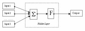
Figure 1 Artificial Neuron with Activation Function.
summed up. The summation is termed as NET and must be calculated for each neuron(the hidden layer/output layer nodes). After NET is calculated, an activation function F is applied to modify it, thereby producing the signal OUT. This output OUT is compared with the target output provided to the network and the difference(error) is back-propagated to modify the weights in the network. This process of learning continues until the error minimizes to a desired value. The present form of back propagation algorithm is developed by Rumelhart et al.(1986).
3.2 Procedure of Study
This section gives an outline of the general procedure to carry out the modeling with neural networks.
I. The NN model in this study have several inputs of upward radiance reflectance and a single output of either Chl.a or SS concentration. Out of the 29 data set available, 20 of them is selected as training data to the network and the rest is used as validation data for examining the performance of the trained model. Selection of training data is done by first arranging the entire data set in decreasing order of Chl.a (or SS) concentration and then, starting from the top, picking up every two values and leaving one as validation data.
II. Upward radiance reflectance data taken with the spectro-radiometer is available for the wavelength range [400-848]nm with an interval of 2nm. Six sets of combinations of wavelengths that best represent the concentration of Chl.a and SS are selected as listed below. Input and validation data set for all the 6 combinations are created.
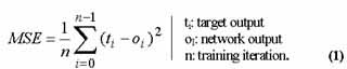
III. The NN model in this study uses only one hidden layer. It has been proven that any function, no matter how complex, can be represented by a neural network with one hidden layer (Masters, 1993). The activation function (F) used is the binary sigmoid (Fig.2) with slope parameter 'g'. All the data output data are scaled in the range [0.1,0.9] to match with the range of activation function, [0,1]. Training of the NN model is performed on data for each Combination set with varying number of hidden layer nodes to find the best one giving faster learning and better convergence. Training rate is varied as the training progresses starting with a value of 0.3. The training error is measured with study Mean Square Error (MSE) [Eqn.1]. It is found that, the NN overfits the training values if training is performed until the MSE flattens down. Hence, the RMS (root-mean-square) error of the training testing set (in our case, the validation set) is calculated in each pass of
training and the training is terminated as soon as it reaches the minimum. Slope parameter 'g' is kept constant throughout the training at 3. Finally, the trained model is subjected to the validation data set.
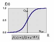
Figure 2: Binary Sigmoid Function
4. RESULTS AND APPLICATION
4.1 Regression Analysis
To compare the ability of neural networks with conventional methods of water quality estimation Multiple regression analysis is performed on all the combinations of data. The dependent variable is either the concentration of Chl.a or SS and the independent variable being the upward radiance reflectance values used as training data in case of NN. Also, the coefficient of determination (R2) and the error in the dependent parameter estimate [the root mean square (RMS) error in this study] have been calculated for both the regression and NN.
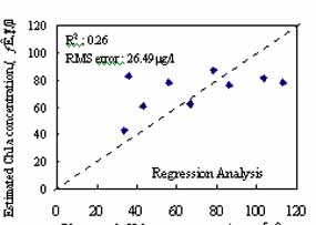
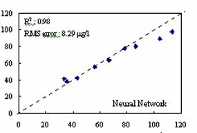
Figure 3. Observed .vs. Estimated Chl.a concentration by Regression Analysis and Neural Network
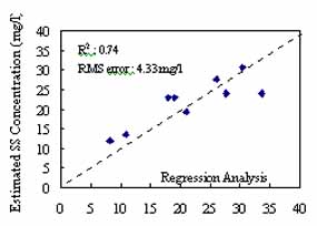
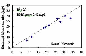
Figure 4. Observed .vs. Estimated SS concentration by Regression Analysis and Neural Network
As a whole for all the combinations, while estimating Chl.a, the RMS error for regression comes out to be 3-4 times than that of NN. However, the difference of RMS errors was not much in case of estimation of SS and NN showing up with better performance. The results (for all combinations) show that, the NN could not predict the high Chl.a concentration quite satisfactorily as expected. This may be due to limited number of data set used in this study or because of the complex behavior of the lake water containing other components contributing to the lake water color such as Chromophoric Dissolved Oxygen Material(CDOM). Combination set 6 and Combination set1 gave best results in predicting the Chl.a and SS concentration respectively for the validation data set.
The trained and validated NN model of Combination set 6 is selected for application to CASI data. Figure 3 and figure 4 shows the NN and regression results for the same with corresponding RMS error and R2 values.
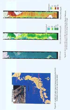
4.2 Application to CASI image
CASI (Compact Airborne Spectrographic Imager) image of lake Kasumi Gaura was taken on 5th of Sept, 1996. It has 96 layers(bands) with spatial resolution of 5m x 3.5 m. 1 CASI DN = 0.001SRU. Data for 10 layers, namely 6, 7, 8, 47, 48, 49, 52, 55, 59 and 62 are sorted out for estimation of Chl-a and SS, as their central wavelengths coincide with that of the Combination set 6 selected for application. To convert the radiance values to reflectance values (to apply the NN model), regression is done between radiance and reflectance values for 3 locations over the lake (plus one on the ground/concrete), the in-situ data for which was taken on the same as CASI. With this regression all the radiance values are converted to corresponding reflectance for input to the NN model. Mean radiance of a 5 x 5 pixel area in the CASI image is taken for representation of each point. Figure 6 in the next page show the spatial distribution of Chl.a and SS concentration in the lake Kasumi Gaura estimated by the NN model.
In a same similar manner, the NN model can be applied to other satellite sensor images such as Landsat TM to get a better and bigger picture of distribution of Chl-a and SS at the lake site.
5. Conclusion
The Neural Network model was able to model the transfer function to a much higher accuracy than multiple regression analysis as expected. The performance of the NN model varies with varying number of hidden layer nodes. The model could not represent the higher values of Chl-a satisfactorily. For a more effective and accurate model to represent the water quality of the site under investigation, the author proposes collection of larger data set including measurements of other primary components believed to contribute to the lake water color such Chromophoric dissolved oxygen material(CDOM) in coincidence with overpass of modern satellite sensor(such as Landsat TM or SeaWIFS).
References
Abstract
Two important parameters for monitoring water quality of inland water bodies are the concentrations of Chlorophyll a (Chl.a) and Suspended Sediment (SS) in the surface water. Due to the optically complex nature of inland water with high turbidity and dissolved organic matter this task becomes quite difficult in comparison to Case-I water. Neural Network have proven its ability successfully in modeling a variety of geophysical transfer function. A Back-Propagation Neural Network (BPNN) model with one hidden layer is employed for modeling the transfer function between the chlorophyll a and sediment concentrations and in situ upward reflectance radiance taken with a spectro-radiometer at the Lake Kasumi Gaura of Japan. The inputs to the network model are the in-situ upward radiance taken all over the Lake Kasumi Gaura and the outputs are the concentrations of Chl.a and SS. The trained and validated model is used to get the spatial distribution of Chl.a and sediment concentrations at the lake Kasumi Gaura using CASI(Compact Airborne Spectrographic Imager) imagery. The Neural Network model was able to model the transfer function to a much higher accuracy than multiple regression analysis. In case of Chl.a estimation, the RMS error for the neural network was 8.29mg/l, whereas the same for regression analysis were 26.498.29mg/l.. However, in case of estimation of SS by regression RMS errors was 3.94mg/l, whereas by Neural Network RMS error came out to be 2.90mg/l..
1. Introduction
Lake Kasumi Gaura is the second largest lake in Japan located about 60 km northeast of Tokyo.. It is a monomictic lake with average depth of about 4 m.. It faces acute problems of eutrophication and heavy sedimentation every year. The lake houses several important cities/towns around its bank which effect or are being effected by the water quality of the same. Keeping in view this very important fact and other, it becomes necessary to parameterize and estimate the water quality parameters as accurately as possible for effective and correct investigation of the present situation and possible solutions. The main factors effecting the water quality of lakes include the concentrations of Chlorophyll-a(Chl.a) and Suspended Solid(SS). This study tries to find a way to effectively estimate these two water quality parameters in the Lake Kasumi Gaura. Present day remote sensing makes it possible to monitor the Chl.a and SS concentration in wide spatial scale. Oki(1997) have developed spatial concentration maps for Chl.a and SS in Lake Kasumi Gaura using Landsat-TM and regression analysis. The authors believed that, conventional techniques like regression can not model the transfer function effectively in complex waters. The study is a result to eliminate this very drawback.
This study employs Neural Networks (NN) as a tool for effectively model the transfer function of Chlorophyll and Suspended Solid in the water of Lake Kasumi Gaura. The model is then is used in CASI image taken at the lake to get the picture of Chl.a and SS distribution.
2. In Situ Data
Water Quality samples for concentrations of Chl.a and SS were collected in the waters of Lake Kasumi Gaura by Oki(1997) for a total of 29 locations spread over the lake. Out of these 29 data set, data for 20 locations were collected on 10th Sept., 1993, 6 locations were collected on 22nd of April, 1994 and the data at remaining 3 locations were collected on 5th of September, 1996, coinciding with the CASI flight over the lake. Measurements of water leaving radiance reflectance at the water surface were also done at all the 29 locations with a spectro-radiometer.
3. Neural Networks
3.1 Background
The idea of Neural Networks (NN) came from the basic structure of functioning of the human brain. In the modern field of science and engineering, NN has strengthened their importance with numerous applications ranging from pattern recognition, fields of classification etc. There are different kind of NN available depending on the task to be performed. In this study the neural network used is Multi layer Feed-Forward type employing back-propagation of Error, simply called Back-Propagation Neural Network.(BPNN). Fig.1 Shows the fundamental building block for a back propagation network.. A set of inputs is applied is applied to the network. Each of these is multiplied by a weight, and the products are
Figure 1 Artificial Neuron with Activation Function.
summed up. The summation is termed as NET and must be calculated for each neuron(the hidden layer/output layer nodes). After NET is calculated, an activation function F is applied to modify it, thereby producing the signal OUT. This output OUT is compared with the target output provided to the network and the difference(error) is back-propagated to modify the weights in the network. This process of learning continues until the error minimizes to a desired value. The present form of back propagation algorithm is developed by Rumelhart et al.(1986).
3.2 Procedure of Study
This section gives an outline of the general procedure to carry out the modeling with neural networks.
I. The NN model in this study have several inputs of upward radiance reflectance and a single output of either Chl.a or SS concentration. Out of the 29 data set available, 20 of them is selected as training data to the network and the rest is used as validation data for examining the performance of the trained model. Selection of training data is done by first arranging the entire data set in decreasing order of Chl.a (or SS) concentration and then, starting from the top, picking up every two values and leaving one as validation data.
II. Upward radiance reflectance data taken with the spectro-radiometer is available for the wavelength range [400-848]nm with an interval of 2nm. Six sets of combinations of wavelengths that best represent the concentration of Chl.a and SS are selected as listed below. Input and validation data set for all the 6 combinations are created.
| Combination set 1: | 440 674 676 700 724 726 | [nm] : 6 inputs (reflectance) |
| Combination set 2: | 440 675 700 725 | [nm] : 4 inputs (reflectance) |
| Combination set 3: | 440 675 676 700 | [nm] : 4 inputs (reflectance) |
| Combination set 4: | 675 676 700 725 | [nm] : 4 inputs (reflectance) |
| Combination set 5: | 442 444 446 674 676 678 700 720 740 760 | [nm]: 10 inputs (reflectance) |
| Combination set 6: | 442 446 452 672 678 682 700 720 740 760 | [nm]: 10 inputs (reflectance) |
III. The NN model in this study uses only one hidden layer. It has been proven that any function, no matter how complex, can be represented by a neural network with one hidden layer (Masters, 1993). The activation function (F) used is the binary sigmoid (Fig.2) with slope parameter 'g'. All the data output data are scaled in the range [0.1,0.9] to match with the range of activation function, [0,1]. Training of the NN model is performed on data for each Combination set with varying number of hidden layer nodes to find the best one giving faster learning and better convergence. Training rate is varied as the training progresses starting with a value of 0.3. The training error is measured with study Mean Square Error (MSE) [Eqn.1]. It is found that, the NN overfits the training values if training is performed until the MSE flattens down. Hence, the RMS (root-mean-square) error of the training testing set (in our case, the validation set) is calculated in each pass of
training and the training is terminated as soon as it reaches the minimum. Slope parameter 'g' is kept constant throughout the training at 3. Finally, the trained model is subjected to the validation data set.
Figure 2: Binary Sigmoid Function
4. RESULTS AND APPLICATION
4.1 Regression Analysis
To compare the ability of neural networks with conventional methods of water quality estimation Multiple regression analysis is performed on all the combinations of data. The dependent variable is either the concentration of Chl.a or SS and the independent variable being the upward radiance reflectance values used as training data in case of NN. Also, the coefficient of determination (R2) and the error in the dependent parameter estimate [the root mean square (RMS) error in this study] have been calculated for both the regression and NN.
Figure 3. Observed .vs. Estimated Chl.a concentration by Regression Analysis and Neural Network
Figure 4. Observed .vs. Estimated SS concentration by Regression Analysis and Neural Network
As a whole for all the combinations, while estimating Chl.a, the RMS error for regression comes out to be 3-4 times than that of NN. However, the difference of RMS errors was not much in case of estimation of SS and NN showing up with better performance. The results (for all combinations) show that, the NN could not predict the high Chl.a concentration quite satisfactorily as expected. This may be due to limited number of data set used in this study or because of the complex behavior of the lake water containing other components contributing to the lake water color such as Chromophoric Dissolved Oxygen Material(CDOM). Combination set 6 and Combination set1 gave best results in predicting the Chl.a and SS concentration respectively for the validation data set.
The trained and validated NN model of Combination set 6 is selected for application to CASI data. Figure 3 and figure 4 shows the NN and regression results for the same with corresponding RMS error and R2 values.
4.2 Application to CASI image
CASI (Compact Airborne Spectrographic Imager) image of lake Kasumi Gaura was taken on 5th of Sept, 1996. It has 96 layers(bands) with spatial resolution of 5m x 3.5 m. 1 CASI DN = 0.001SRU. Data for 10 layers, namely 6, 7, 8, 47, 48, 49, 52, 55, 59 and 62 are sorted out for estimation of Chl-a and SS, as their central wavelengths coincide with that of the Combination set 6 selected for application. To convert the radiance values to reflectance values (to apply the NN model), regression is done between radiance and reflectance values for 3 locations over the lake (plus one on the ground/concrete), the in-situ data for which was taken on the same as CASI. With this regression all the radiance values are converted to corresponding reflectance for input to the NN model. Mean radiance of a 5 x 5 pixel area in the CASI image is taken for representation of each point. Figure 6 in the next page show the spatial distribution of Chl.a and SS concentration in the lake Kasumi Gaura estimated by the NN model.
In a same similar manner, the NN model can be applied to other satellite sensor images such as Landsat TM to get a better and bigger picture of distribution of Chl-a and SS at the lake site.
5. Conclusion
The Neural Network model was able to model the transfer function to a much higher accuracy than multiple regression analysis as expected. The performance of the NN model varies with varying number of hidden layer nodes. The model could not represent the higher values of Chl-a satisfactorily. For a more effective and accurate model to represent the water quality of the site under investigation, the author proposes collection of larger data set including measurements of other primary components believed to contribute to the lake water color such Chromophoric dissolved oxygen material(CDOM) in coincidence with overpass of modern satellite sensor(such as Landsat TM or SeaWIFS).
References
- Keiner, L.E. and Yan, X.H., 1998. A Neural Network Model for
Estimating Sea Surface Chlorophyll and Sediments from Thematic Mapper
Imagery. Remote Sensing of Environment, Elsevier, 66:153-165.
- Masters, T, 1993. Practical Neural Network Recipes in C++. Academis
Press, 491pp.
- Oki, H, 1997. Study of Lake basin Land use and its Impact on Lake
Water Quality. Doctoral Thesis, University of Tsukuba Library, 141pp.
- Rumelhart, D., Hinton, G.E., and Williams, R.J., 1986a. Learning Representations by back-propagating errors. Nature (London), 323, pp533-536.