| GISdevelopment.net ---> AARS ---> ACRS 2000 ---> Oceanography |
Comparative Performance of
SST Algorithms In the Tropical Ocean Using OCTS Data
K. Abdullah, M. Z. MatJafri
and N. M. Saleh
Universiti Sains Malaysia 11800 Penang, Malaysia
Tel: 604-6577888 Fax: 604-6579150
E-mail:khirudd@usm.my, mjafri@usm.my, nasirun@usm.my
A. Bahari
Malaysian Meteorological Service 46667 Petaling Jaya
Selangor, Malaysia
Tel: 603-7569422 Fax: 603-7550964
E-mail:alui@kjc.gov.my
Keywords:algorithm, emissivity, sea surface
temperature, transmittanceUniversiti Sains Malaysia 11800 Penang, Malaysia
Tel: 604-6577888 Fax: 604-6579150
E-mail:khirudd@usm.my, mjafri@usm.my, nasirun@usm.my
A. Bahari
Malaysian Meteorological Service 46667 Petaling Jaya
Selangor, Malaysia
Tel: 603-7569422 Fax: 603-7550964
E-mail:alui@kjc.gov.my
Abstract
A two-channel algorithm for measuring sea surface temperature (SST) using non-regression coefficients was applied to the Ocean Colour Temperature Scanner (OCTS) data from the Advanced Earth Observation Satellite (ADEOS). The algorithm is based on the fact that the recorded infrared signal at the sensor is composed of three terms, namely, the surface emission, the upwelling radiance emitted by the atmosphere, and the downwelling atmospheric radiance that is reflected at the sea surface. This algorithm requires the atmospheric transmittance values of two thermal bands. In this study the transmittance function for each band was modeled using the MODTRAN code and radiosonde data. The expression of transmittance as a function of zenith view angle was obtained for each channel through regression of the MODTRAN output. The in-situ data (ship collected SST values) were used for verification of results. Contour maps of the in-situ SST values were generated because clouds covered the measured locations. Cloud contaminated pixels were masked out using the standard procedures. The cloud free pixels were extracted and converted to brightness temperature values and then substituted in the proposed algorithm. The appropriate transmittance value for each channel derived earlier was then assigned in the calculation. The correlation coefficients and the root-mean-square deviations between the computed and the ship-collected values were determined. The results were also compared with the results from OCTS multichannel sea surface temperature (MCSST) algorithm. The performance of this algorithm is comparable with the established OCTS algorithm. SST map was created and comparison with the OCTS algorithm generated map was made.
1.0 Introduction
Sea surface temperature (SST) algorithms have been determined by two basic techniques: i) regression between coincident satellite brightness temperatures and surface measurements, and ii) theoretical atmospheric transmission model with a set of representative vertical profiles of atmospheric temperature and absorbing constituents is used (Barton 1995). Various algorithms for performing this task have been developed; these include the single infrared channel method, the multichannel method and the multiangle method. The operational SST algorithms using AVHRR data established their coefficients through regression techniques. Recently, the MCSST algorithm has been developed by NASDA for OCTS data using similar approach.
Application of regression technique requires a sufficient amount of coincident in-situ data with the remotely sensed data. The requirement is not easily achievable in the equatorial region due to unfavorable sky conditions. Therefore in this study, the algorithm that has been derived theoretically which does not require in-situ SSTs for calibration was used. This algorithm is designed to measure SST using thermal images from any satellite. The purpose of this study is to test our developed algorithm using OCTS data sets. The performance of this algorithm was compared with the NASDA MCSST and in-situ data.
2.0 Data Sets
Three OCTS TI level 1B scenes covering the South East Asia region were selected based on availability of cloud free pixels. They were captured (daytime) by ADEOS satellite on 22 March 1997, 21 April 1997 and 13 June 1997. In-situ SST data collected by sea cruises (under the Voluntary Observing Ship Programme of the World Meteorological Organization) on these dates were supplied by the Malaysian Meteorological Service.
3.0 Data Calibration
The conversion from digital number, DN, to radiance, L (mW cm-2 str-1 mm-1) was performed using the information given by NASDA. The radiance values were converted to brightness temperature values, T (K), for band 10, 11 and 12 of OCTS data by using the published conversion table (table IX of Shimada 1998). Analysis of the tabulated values for the temperature range from 273 K to 315 K, showed that the relationship could be accurately described by the polynomial equation
The coefficients were determined through regression.
4.0 Cloud Masking Techniques
The thermal infrared bands were used because the near infrared bands contained some noise problems. Three techniques were employed, (a) the infrared threshold test or gross cloud check, (b) the spatial coherence technique, and (c) the channel difference (Saunders and Kriebel, 1988). For each image date, several small sub-scenes (channels 10,11,12) containing clouds and cloud free water pixels were extracted for detailed study using each technique mentioned above. Digital numbers (DN) were used in the analysis instead of brightness temperature values to simplify the data processing. After the data were passed through the series of tests described earlier, the combined cloud masks were finally obtained.
5.0 Sea Surface Temperature Algorithm
Based on the radiative transfer equation in the atmosphere for a cloud free atmosphere under local thermodynamic equilibrium, a single channel algorithm can be derived for measuring sea surface temperature for infrared band i.
where Ti = brightness temperature of band i
Ta= temperature of atmosphere
D(Ti= Li/[dL/dT(Ti)]
ai = eiti
bi= (1-ti)(1 + ti - eiti)
ei= emissivity of sea water in band i
ti= atmospheric transmittance
By writing the equation for another band j, a split window expression or dual-channel algorithm (Abdullah 1994) for measuring sea surface temperature, Ts can finally be obtained
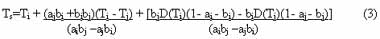
The algorithm requires two environmental parameters, (i) the atmospheric transmittance and (ii) the emissivity of seawater. The transmittance was modelled using the MODTRAN code. Radiosonde data acquired on the dates of OCTS scenes were used in the MODTRAN calculation for the atmospheric model. For each channel, the view angle from the top of the absorbing atmosphere was varied in steps of 5 degrees from 0 to 65 degrees. The average transmittance values and their corresponding zenith angles were noted. Inspection of the results suggests that the relation can be approximated by the expression
where q is the satellite zenith angle at the pixel location. The coefficients were determined from regression analysis.
Various emissivity values have been used in SST retrieval algorithms. The earlier algorithms used e = 1. Singh (1984) assumed 0.98 in his calculation. The spectral dependence of emissivity, where e4=0.992 and e5=0.989 was considered by Becker and Li (1990).
6.0 Computation of Sea Surface Temperature
Equation (3) can be used for atmospheric correction at any satellite angle or on a pixel-by-pixel basis. Cloud free seawater pixels for bands 10, 11 and 12 were extracted for SST retrieval. The digital numbers were converted to brightness temperatures and their corresponding zenith angles were calculated. The emissivity was assumed to be 0.96 (the value given in the MODTRAN manual for 12mm) in both bands. Appropriate transmittance function derived earlier was used for each image date. Having determined the transmittance as a function zenith angle and the emissivity for seawater for each band, equation (3) can be applied to measure SST
7.0 Comparison With NASDA MCSST Algorithm
The Multichannel Sea Surface Temperature algorithm developed by NASDA (Sakaida et al. 1998) is expressed as
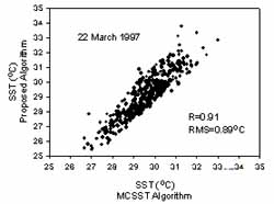
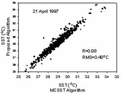
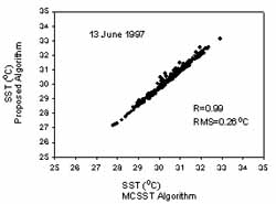
The SST values computed using the proposed algorithm were then compared with the values retrieved using the MCSST algorithm. The outputs from these algorithms were correlated. The RMS deviations of the computed values using the proposed algorithm from the MCSST outputs were estimated. Table 1 and the set of graphs in Figure 1 show the results of the analysis. With these data sets the present algorithm has shown comparable performance with the established algorithm produced by NASDA.
| R | RMS(°C) | |
| 22 March 1977 | 0.91 | 0.89 |
| 21 April 1977 | 0.98 | 0.48 |
| 13 June 1977 | 0.99 | 0.26 |
 |
 |
| (a) | (b) |
 | |
| (c) | |
Figure 1 Comparison of the proposed algorithm with the MCSST algorithm (a) 22 March1997, (b) 21 April1997and (c) 13 June 1997
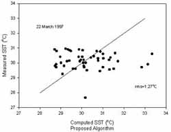
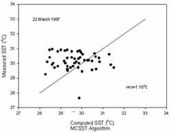
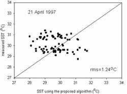
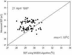
8.0 Validation of Results
The in-situ data collected within the region of interest were used for verification of the retrieved SST values. From the analysis, unfortunately, we discovered that all the in-situ points were located on cloudy pixels. Measured SST values were interpolated spatially by plotting contour maps of the in-situ data. These maps were used to verify the computed SST values. The locations of the cloud free pixels were determined and the corresponding in-situ values were read from the map. The 22 March 1997 and 21 April 1997 cloud free pixels areas occurred within the generated contour maps. The results of the verification using the proposed algorithm and the MCSST algorithm are listed in Table 2. Figure 2 shows their scatter plots.
| Proposed algorithm (RMS,°C) | MCSST (RMS,°C) | |
| 22 March 1977 | 1.27 | 1.10 |
| 21 April 1977 | 1.24 | 1.18 |
 |
 |
| (a) | (b) |
 |
 |
| (c) | (d) |
Figure 2 Comparison of computed SST values with the measured values (a) the proposed algorithm (22/3/1999), (b) MCSST algorithm (22/3/1999), (c) proposed algorithm (21/4/1999) and (d) MCSST algorithm (21/4/1999)
9.0 Generation of SST Maps
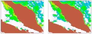
Both algorithms were applied to the thermal infrared bands to generate SST maps. The land and cloud areas were masked out. Figure 3 shows the generated SST maps for the image date of 21 April 1997 using the two algorithms. Similar SST patterns are shown by both images.
10.0 Conclusion
The results of the study indicated that the performance of the developed algorithm is comparable to the established NASDA MCSST algorithm. However, this algorithm requires only two thermal infrared bands instead of three bands used by NASDA. This algorithm takes into account of the local atmospheric condition. The retrieved SST values are highly correlated with the NASDA MCSST computed values. The computed values using the proposed algorithm deviated by a small amount from the MCSST retrieval values. The typical SST values in the studied region were between 28°C to 31°C. However very little points having these values were used in NASDA calibration analysis and some of these points showed higher in-situ values than the computed values. At higher temperatures, proposed algorithm gave slightly higher values than those computed using NASDA MCSST. Based on the analysis, proposed algorithm is capable to produce reliable results. The present study has indicated that it is possible to use this algorithm globally. It requires the knowledge of the atmospheric transmittance at the study location. Coincident SST values are needed for more accurate verification. This will be verified by pursuing further research.
 | |
| (a) | (b) |
Figure 3 SST maps on 21 April 1997 using (a) the proposed algorithm and (b) NASDA algorithm (colour code: blue 28-29°C, green 29-30°C, yellow 30-31°C, orange > 31°C, white for cloud and brown for land areas)
Acknowledgments
This study is partially supported by NASDA through the joint NASDA-ESCAP project. Thanks are extended to RESTEC, the Universiti Sains Malaysia and the Malaysian Meteorological Service.
References
- Abdullah, K., 1994. The use of satellite data in studying geophysical and biological aspects of coastal waters. PhD Thesis, University of Dundee.
- Barton, I. J., 1995. Satellite derived sea surface temperatures: Current status. Journal of Geophysical Research, 100: 8777-8790.
- Becker, F. and Li, Z. L., 1990. Towards a local split window method over land surfaces. International Journal of Remote Sensing, 11:369-394.
- Sakaida, F., Moriyama, M., Murakami, H., Oaku, H., Mitomi, Y., and Kawamura, H., 1998. The sea surface temperature product algorithm of the Ocean Colour Temperature Scanner (OCTS) and its accuracy. Journal of Oceanography, 54: 437-442.
- Saunders, R. W. and Kriebel, K. T., 1988. An improve method for detecting clear sky and cloudy radiances from AVHRR data. International Journal of Remote Sensing, 9: 123?150.
- Shimada, M., 1998. A cal/Val Report on the OCTS version 3 product.
- Singh, S. M., 1984. Removal of atmospheric effects on a pixel by pixel basis from the thermal infrared data from instruments on satellites. The Advanced Very High Resolution radiometer (AVHRR). International Journal of Remote Sensing, 5: 161?183.