| GISdevelopment.net ---> AARS ---> ACRS 2000 ---> Mapping from Space & GPS |
Performance Evaluation Of Rtk
Gps Without Sa Effect
Jenn-Taur LEE Wen-Feng
CHEN
Department of Surveying and Mapping Engineering
Chung Cheng Institute of Technology
National Defense University
Tahsi, Taoyuan Taiwan 33509
Tel: 886-3-380-0364 Fax: 886-3-390-7810
Email:jtlee@mail.ccit.edu.tw
Keywords: Global Positioning System, Selective
Availability, Real Time Kinematic GPSDepartment of Surveying and Mapping Engineering
Chung Cheng Institute of Technology
National Defense University
Tahsi, Taoyuan Taiwan 33509
Tel: 886-3-380-0364 Fax: 886-3-390-7810
Email:jtlee@mail.ccit.edu.tw
Abstract
The policy of Selective Availability (SA) was endorsed in order to artificially widen the gap between the civilian and military positioning services. SA is an intentional degradation of the accuracy of global positioning system (GPS) horizontal positioning to 100m and height determination to 150-170m at the 95% confidence level, for standard positioning service (SPS) users. SA has been implemented since March 25, 1990, and consists of two different components.
Firstly, the so-called epsilon ( e ) component consists of the truncation of the orbital information transmitted within the navigation message so that the WGS84 coordinates of the satellites cannot be computed correctly. Secondly, the so-called delta ( d ) component which is achieved by dithering the satellite clock output frequency. The varying error in the satellite clock's fundamental frequency has the direct impact on both the pseudo-ranges and carrier phase observations. The variations in range have amplitudes of as much as 50m, with periods of several minutes. Fortunately, SA was discontinued on May 2, 2000 that should make GPS more responsive to civil and commercial users.
The objective of this study is to investigate the performance of real time kinematic (RTK) GPS without SA effect, since RTK GPS is widely taken in engineering and geographical information system (GIS) uses. The experiment was accomplished in an existed network that consists of 31 control points, which was surveyed with RTK GPS in addition static GPS, differential GPS, and single point positioning before and after SA effect turned off. EDM and leveling surveying was also done at the same network. Furthermore, the statistical analyses of horizontal and vertical vectors, baseline length, and height difference were completed and will be presented in the article.
1. Introduction
GPS is a dual-use system, providing highly accurate positioning and timing data for both military and civilian users. There are more than 4 million GPS users world wide, and the market for GPS applications is expected to double in the next three years, from 8 billion to over 16 billion. Some of these applications include: air, road, rail, and marine navigation, precision agriculture and mining, oil exploration, environmental research and management, telecommunication, electronic data transfer, construction, recreation and emergency response. GPS has always been the dominant standard satellite navigation system thanks to the U.S. policy of making both the signal and the receiver design specification available to the public completely free of charge. The U.S. previously employed a technique called Selective Availability (SA) to globally degrade the civilian GPS signal. New technologies demonstrated by the military enable the U.S. to degrade the GPS signal on a regional basis. GPS users worldwide would not be affected by regional, security-motivated, GPS degradations, and businesses reliant on GPS could continue to operate at peak efficiency [Leick, 1996]. The technology that makes this extraordinary technology possible grows directly from past research investments in basic physics, mathematics, and engineering supported from U.S. Federal agencies over a period of decades.
GPS works because of super reliable atomic clocks-no mechanical device could come close. These clocks resulted from gifted physics and creative engineering that managed to package devices which once filled large physics laboratories into a compact, reliable, space-worthy device. The improved, non-degraded signal will increase civilian accuracy by an order of magnitude, and have immediate implications in areas such as car navigation, emergency services, recreation, and others. In addition to more accurate position information, the accuracy of the time data broadcast by GPS will improve to within 40 billionths of a second. Such precision may encourage adoption of GPS as a preferred means of acquiring Universal Coordinated Time (UTC) and for synchronizing everything from electrical power grids and cellular phone towers to telecommunications networks and the Internet [Teunissen, 1998]. For example, with higher precision timing, a company can stream more data through a fiber optic cable by tightening the space between data packages. Using GPS to accomplish this is far less costly than maintaining private atomic clock equipment.
2. Error Sources Of GPS
The accuracy with which a GPS receiver can determine position and velocity and synchronize to GPS time is dependent on a number of factors. GPS error sources are allocated into three categories: the space segment, control segment, and user segment. The error components that comprise these segment, as well as an estimate of the one-sigma value of each component is given in Table 1. The most dominant error source by far is Selective Availability (SA) that produces a one-sigma error of 32.3 meters. These error sources are for the civilian coarse/acquisition (C/A) code. The effective accuracy of the pseudorange value is termed the user-equivalent range error (UERE). The system UERE is the root sum square (RSS) of the individual error components. As shown in Table 1, the one-sigma UERE is reduced from 33.3 m with SA to only 8 m when SA is removed. Further reduction in the UERE can be obtained with the proposed 2nd and 3rd civilian frequencies to correct for ionospheric delay. A UERE of 6.6 m was examined to account for the ionospheric correction, as well as a UERE of 3.8 m that includes additional benefits of GPS modernization [Kaplan, 1996].
A more conservative user error budget also was examined to account for larger receiver noise and ionospheric errors. The troposphere and multipath errors also were modified to agree with the supplemental GPS Minimum Operational Performance Standards (MOPS). This error budget, shown in Table 2, results in a one-sigma pseudorange error of 12.5 m without SA. The root sum square of the receiver noise, multipath, and interchannel bias equals 5 meters which is consistent with the value in the current Wide Area Augmentation System (WAAS) MOPS. A one-sigma pseudorange error of 12.5 meters for GPS without SA was adopted by RTCA SC-159 Working Group 2 for inclusion in the WAAS MOPS. As shown in Equations (1) and (2), the magnitude of the horizontal protection level is directly related to the standard deviation of the pseudorange error. This reduction of horizontal protection level (HPL) naturally will translate into a significant improvement in availability. The horizontal protection level is determined by HPL = SFmax bias (1)
Where bias =s Öl (2)
SF is the scale factor, l is the noncentrality parameter of the noncentral chi-square density function, s and is the standard deviation of the satellite pseudorange error.
| Segment Source | Error Source | GPS 1s Error(m) with SA | GPS 1s Error(m) without SA |
| Space | Satellite Clock Stability Satellite Perturbations Selective Availability Other (thermal radiation,etc.) |
1.0 32.3 0.5 |
1.0 - 0.5 |
| Control | Ephemeris Prediction Error Other (thruster performance, etc.) |
0.9 |
0.9 |
| User | Ionospheric Delay Tropospheric Delay Receiver Noise and Resolution Multipath Other (interchannel bias, etc.) |
1.5 1.5 2.5 0.5 |
1.5 1.5 2.5 0.5 |
| System UERE | Total (RSS) |
|
|
| Error Source | GPS 1s Error (m) without SA |
| Ionospheric Delay Tropospheric Delay Receiver Noise and Resolution Multipath Other (interchannel bias, etc.) |
2.0 4.8 1.2 0.5 |
| System UERE (RSS) |
|
Space and control segment errors remain the same (without SA).
3. Methodology of RTK GPS
The key of RTK GPS positioning is the ambiguity solution in the movement, when the dual frequency phase measurements of master and rover stations are put together through the radio communication. If the position of master station is known, then the position of rover station is solved by double differencing algorithm, so the merits of RTK GPS are rapid positioning and cm level of accuracy [Langley, 1998; Leick, 1996].
The phase ambiguity could be resolved in a short period and only few epoch of observations, which is contributed by the full constellation of GPS satellites, the complete full wavelength of dual frequency receiver, and the advanced decoding ability. Therefore, the ambiguity function method, the fast ambiguity resolution approach, the least squares ambiguity search technique, the fast ambiguity search filter, and the on-the-fly approach are commonly adopted to gain the integer ambiguity [Abidin, 1994].
The general procedures for estimating the ambiguity are listed as the followings:
- initial location estimation;
- search space generation;
- phase ambiguity search;
- phase ambiguity verification.
4. Description of Experiments
The experiments performed on campus of Chung Cheng Institute of Technology, National Defense University. The GPS control network consisted of 31 points and the situation of control points is displayed in Figure 1. Since point A001 is considered as the fixed point for static GPS surveying, the tasks of baseline vector processing and network adjustment were done by software package. The three-dimension outcomes taken from the network adjustment are used for reference standard. Moreover, the RTK GPS accomplished over 14 points with SA and 30 points without SA. The instruments employed include Ashtech GPS receivers and Leica RTK GPS positioning system. In addition, the software packages involved GeoGenius from Spectra Precision, SKI from Leica, Excel from Microsoft, and Survey generated from this research group.
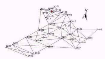
Figure 1 Experimental Network
5. Performance Evaluation of RTK GPS
The evaluation tasks will be separated into RTK GPS with SA and without SA cases.
5.1 RTK GPS with SA
The static GPS surveying transacted and the outcomes are deliberated as the known facts for evaluating the capability of RTK GPS technique. Eventually, 14 points in the experimental network occupied with RTK GPS when B001 was fixed, but points B031, B033, B036, B037, and C030 were phased out during the statistical analyzing task because of no outcome appeared that may caused by the thoughtfully obstruction and the bad signal. The statistical analysis of geographical coordinates is listed in Table 3. The difference of latitude, longitude, and height does range about 1arc-second, 0.02arc-second, and 0.9m, respectively. In addition, the average deviation is around 0.1arc-second in latitude, 0.001arc-second in longitude, and 0.09m in height. In fact, the significant latitude deviation does happen in B010 and B035; the notable longitude deviation does occur in B035; the noted height deviation does appear in B035. If B010 and B035 points are not included, then the consequence may be more reasonable that is almost 1cm in horizontal vector and 2cm in vertical vector. Table 4 is the description of baseline length deviation between RTK and static GPS. The deviation range and average deviation are about 0.9m and 0.01m, respectively. The evidence of portion baseline length is not enough stability that is similar to the previous remark. Besides, the lager deviation is arisen in the longer baseline.
|
|
|
|
|
| B010 |
|
|
|
| B013 |
|
|
|
| B032 |
|
|
|
| B034 |
|
|
|
| B035 |
|
|
|
| BL01 |
|
|
|
| C026 |
|
|
|
| C027 |
|
|
|
| C031 |
|
|
|
| Max |
|
|
|
| Min |
|
|
|
| Mean |
|
|
|
| RMS |
|
|
|
|
|
|
|
|
|
|
|
|
|
|
|
|
|
|
|
|
|
|
|
|
|
|
|
|
|
|
|
|
|
|
|
|
|
|
|
|
|
|
|
|
|
|
|
|
|
|
|
| |
|
|
|
| |
|
|
|
| |
|
|
|
| |
5.2 RTK GPS without SA
After SA was turned off, the static and RTK GPS re-occupied the experimental network. Through the similar baseline processing and network adjustment, the outcomes of static GPS are still contemplated as the reference standard to judge the performance of RTK GPS without SA effect. The statistical analysis of TM 2° coordinates is listed in Table 4 that the deviation is less than 1cm in east and north directions and below 3cm in height, so the reliability of RTK GPS without SA is meaningful. At that time, the comparison task of RTK GPS with and without SA carried out and the estimated result is displayed in Table 6 that the discrepancy is below 3cm in east and north directions and about 10cm in height. It is compassion that only three points could evolve in the comparison because of satellite constellation and station surroundings.
|
|
|
|
|
|
|
|
|
|
|
|
|
|
|
|
|
|
|
|
|
|
|
|
|
|
|
|
|
|
|
|
|
|
|
|
|
|
|
|
|
|
|
|
|
6. Conclusions
According to the preliminary analysis on horizontal vector, vertical vector and baseline length, the RTK GPS does denote to have the capability of static GPS technique in positioning. In other words, the RTK GPS technique is feasible, effective, and efficient for positioning and other applications, but the stableness is the most concern issue. Obviously, the reliability of RTK GPS could reach the centimeter level that is very near the order of static GPS, but the RTK GPS affected by SA on or off is also limited in centimeter level. The major difficulty of RTK GPS is the obstruction around station and the capability of radio power.
7. References
- Abidin, H.A., 1994. On-the-Fly Ambiguity Resolution. GPS World, No. 4, pp. 47-56.
- Kaplan, E.D., 1996. Understanding GPS Principles and Applications. Artech House, New York.
- Langley, R.B., 1998. RTK GPS. GPS World, No. 9, pp. 70-76.
- Leick, A., 1996. GPS Satellite Surveying. John Wiley & Sons, Inc., New York. pp. 317-409.
- Teunissen, P.J.G., 1998. GPS for Geodesy. Springer-Verlag, New York, pp. 271-318.