| GISdevelopment.net ---> AARS ---> ACRS 2000 ---> Landuse |
Classification of Remotely
Sensed Imagery Using Markov Random Fields
Brandt TSO (Taiwan), Paul
M. Mather(UK)1
Associated Professor, Research Centre, Operation R&D Division
National Defence Management College, National Defence University
Jong-Ho P.O. Box 90046, Taipei
Tel: +886-2-2254-8131 or +886-2-2222-2137 ext 8452, Fax +886-2-2254-8131
E-mai:l brandttso@kimo.com.tw
1Professor, Remote Sensing Society Vice President, School of Geography
University of Nottingham, Nottingham NG7 2RD England
Email: paul.mather@nottingham.ac.uk
Key WordsAssociated Professor, Research Centre, Operation R&D Division
National Defence Management College, National Defence University
Jong-Ho P.O. Box 90046, Taipei
Tel: +886-2-2254-8131 or +886-2-2222-2137 ext 8452, Fax +886-2-2254-8131
E-mai:l brandttso@kimo.com.tw
1Professor, Remote Sensing Society Vice President, School of Geography
University of Nottingham, Nottingham NG7 2RD England
Email: paul.mather@nottingham.ac.uk
Markov Random Field, Genetic Algorithm, Multisource Classification
Abstract
The use of contextual information for modelling the prior probability mass function (generally called the smoothness prior) in the traditional statistical Bayesian classification formula has been widely adopted in recent years. Random field models, especially Markov random fields (MRF), provide a theoretical robust yet mathematical tractable way of coding multisource information and modelling such contextual behaviour. In dealing with remotely-sensed multisource data, the determination of source-weighting and MRF model-related parameters is a difficult task. We've used the genetic algorithm GA to address the parameter estimation issue in a case study over Red Sea Hill, Sudan for lithological type identification (total eight categories were involved in our classification analyses). GA has been proved in many studies to be a powerful, however cost-effective tool for searching optimal solution. The data set used for the experiment includes LANDSAT Thematic Mapper (TM) six-band and Shuttle Image Radar (SIR) L band, C band, and total power multisource data. Three kinds of MRF classification mechanisms known as Iterated Conditional Mode-ICM, Maximiser of Posterior Marginals-MPM, and Line-Process were investigated. It was shown that the incorporation of contextual information leads to impressively improved results (up to 80% of average producer's accuracy was achieved) in comparison with the output derived from traditional non-contextual maximum likelihood classifier (only around 67% of average producer's accuracy was obtained). The resulted classified imagery using context were also found to reveal more patch-like, meaningful patterns. We therefore conclude that incorporating contextual relationship in terms of MRF, with well assignments of model-related parameters and suitable classification algorithms being used, can be a powerful tool for real world, remotely-sensed imagery classification.
Introduction
In recent years, there has been an increasing interest in use of contextual information for modeling the prior probability density function (p.d.f.) (Derin and Elliott, 1987, Dubes and Jain, 1989, Jhung and Swain, 1996, Schistad et al., 1996, Tso and Mather, 1999). Using context to model prior probability to help the interpretation of remotely-sensed imagery is considered as a reasonable procedure, since a pixel classified as "ocean" is likely to be surrounded by the same class and more unlikely to have neighbors from categories such as "pasture" or "forest". In other words, using the concept of context, each pixel is not treated in isolation but as part of a spatial pattern. The relationship between the pixel of interest and its neighbor is therefore not considered to be statistically independent. If context information can be suitably modeled and incorporated with class-conditional p.d.f., then improved classification results can be expected(Li, 1995a, Li, 1995b)..
Discrete random field models, especially the Gibbs Random Fields (GRF) and Markov Random Fields (MRF), have been found to be useful tools for characterizing contextual information and are widely used in image segmentation and restoration(German and German, 1984, German and Gidas, 1991, Tso and Mather, 1999). This study presents some basics ideas of MRF as a framework to model prior probability (and so as to achieve MAP estimate) for remotely-sensed imagery classification.
Theoretical Background
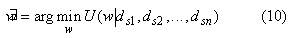
In the interpretation of remotely-sensed imagery, there will be a set of observed feature vectors (e.g. pixel gray value in different bands), d. Traditionally, each pixel r is labeled based on dr alone without considering contextual information. Once the context is included as a prior information and modeled in terms of MRF, current practice is to use a Bayesian formulation to construct the posterior energy and to search the MAP-MRF labeling in terms of energy minimization.
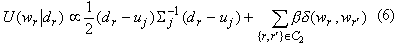
Multisource Posterior Energy
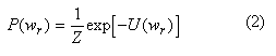
Based on Bayesian formula, the posterior distribution P(w½d) can be expressed as

Recall from (1) that under a pair-site MLL model, the prior probability for pixel r is
where the U(wr) is the prior energy, and is defined as
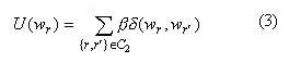
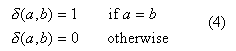
where b £ 0, and define d(wr), wr')) as a step function:
The conditional distribution dr) given the true label wr) is often assumed to be normal. For wr) = label j, the conditional probability which can be formulated as
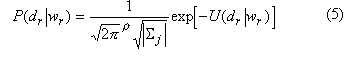
which is the class-conditional energy. By combining (10) and (13), one obtains the posterior energy as
The MAP estimate is equivalent to minimizing the posterior energy.
For multisource classification, in terms of simplicity, we have made a class-conditional independence assumption, i.e.

where dsi is the observation from data source i. Eq. (7) means that we consider the observations from different sources to be conditionally independent. Such an assumption may not be universally valid. However, by adopting this assumption, the mathematical analysis and computation become treatable.
If we take the data-associated reliability factor into account, one simple method is to assign weighting parameters through exponential form, then Eq.(7) can be further refined as

where the
 are the data-associated reliability factor
for the source k. The larger the value of lk the greater the influence of
data source k on the classification process. Eq. (8) indicates that
multisource posterior energy can be expressed as
are the data-associated reliability factor
for the source k. The larger the value of lk the greater the influence of
data source k on the classification process. Eq. (8) indicates that
multisource posterior energy can be expressed as 
Therefore, based on (9), an alternative expression of the MAP-MRF estimation of multisource data is:
where
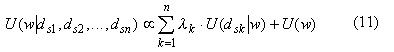
U(w) is defined in (3). Eq. (11) can be regarded as a generalized version of (6).
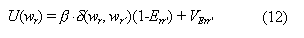
The idea outlined above is mainly designed to achieve a smooth interpretation of remoteing sensing imagery. In practice, the patterns in an image are only piece-wise continuous. That is, discontinuities (i.e. edges between different patches) are naturally to be found within an image. In such cases, the use of a smooth interpolation operation may smear these discontinuities, causing over-smoothing. We are interested here in the method called line-process(Li, 1995b) because it allows us to mark discontinuities and minimize energy simultaneously.
The basic idea of the line-process is quite simple. Once a discontinuity (edge) between two adjacent pixels has been identified, the interaction (i.e. smooth interpolation operation) between these two neighboring pixels should reduced or set off, and it is reasonable to define some other potential to respond to the presence of the edge. Following this logic, the prior energy in (11) can be modified as follows:
Energy Minimization
Once the posterior energy model and the associated parameters have been determined, the next step is to find out the solution (i.e. start classification). As noted previously, a popular method of pixel labeling is to find the MAP estimate using the Bayesian formulation. The MAP approach is also equivalent to a minimum-energy solution in terms of MRF modeling. If the energy function is convex then the MAP-MRF solution can be obtained by using a search approach, such as the gradient descent technique, because there is only one minimum, which is a global one, in the solution space. However, for a non-convex energy function, the solution space may contain several local minimum. In order to obtain a truly MAP estimate, i.e. to find a global minimum, one has to search the full solution space exhaustively.
Three algorithms, known as Iterated Conditional Modes (ICM), Maximiser of Posterior Marginals (MPM), and Line Process have been proposed in the literature to test classification results. All three algorithms are referred to (Li, 1995b). The genetic algorithm was used for search optimal parameter assignments for the developped model.
Experimental Results and Discussions
The study area is located within the Red Sea Hills of Sudan, The categories are shown in Table 1. Based on (12), only pair-sites cliques parameters (i.e. parameter b) are designated non-zero. The range of b was defined as be [5,-5], lke [1,-1]and the isotropy assumption (i.e., single value b, b1 = b2 = b3 = b4, direction independent) was made. The iterations defined for GA in each of three search experiments was 30,000, and each gene was represented by 7 bits, which results in 27.6 (= 242, where each candidate solution contains six genes in which five genes for source weighting parameter candidates and one gene for b; if a non-contextual multisource classification is performed, the search space reduces to 27×5 = 235) choices in GA search space. The parameters determined by GA for both non-contextual and contextual classification are shown in Table 2(a). The parameters shown on row 2 were further used as inputs for MPM classification algorithms. The accuracy acquired is shown in Table 2(b). With the MPM classification algorithm, a range of values for the parameter k and n were tested. We used different combinations of k and n, with k ranging from 1 to 50 and n from 100 to 500. However, no significant difference was found. The classification accuracy in most cases falls within the range of [80, 80.1].
The source-associated weighting factors and clique potential parameters in Table 2(a) show us some interesting properties. The quantity of clique potential parameters determine how strongly the labeling process for the pixel of interest is affected by its neighbours. In order to achieve a good classification result, it is worthwhile to note again that the values of clique potential cannot be chosen without thought, and GA is a suitable tool for overcoming such parameter-determination difficulty. Under the isotropic assumption, a value of -1.5828 of b was detected by GA as the best choice in terms of improving classification accuracy. When the assumption of anistropy is concerned, Table 2 row 3 shows a value of -0.8742 for the second b parameter which indicates a relatively weak contextual effect in terms of vertical orientation. The reason for the lower potential in the vertical direction might be due to the dorminant direction of between-class boundaries as lithological classes have a greater E-W than N-S extent.
The line process mechanism used here is mainly based on (12) using the first order neighbourhood system (4 nearest neighbours) to trigger parameter Err'. However, for parameter VErr', only 4-site cliques are set to be active. Therefore, the value of VErr' will contain 4 choices (i.e., from the 1-edge case to the 4-edge cases). We further define the process rule as follows.
Within a 3 by 3 window, if a discontinuity between the centre pixel r and its upper nearest neighbour has been detected, this will trigger upper left 4 pixels to carry out line process (i.e., to detect edge patterns). If the discontinuity exists between r and its right nearest neighbour, then the line process will be executed for the upper right 4 pixels. Similarly, a discontinuity between the centre pixel r and its lower nearest neighbour will trigger the lower right 4 pixels, and a discontinuity between pixel r and its left nearest neighbour will trigger the lower left 4 pixels. Compared to the contextual classification patterns without incorporating line process, the line process classification appears to generate more small patches (or holes). The presence of these small patches is mainly due to falsely-marked edges.
| Information Class (Number of Pixels) |
|
| TM | SIR-C C-band HH, HV | SIR-C C-band Power | SIR-LL-band HH, HV | SIR-L L-band Power | Clique parameters b | |
| Without Context | 0.8346 | 0.6378 | 0.0709 | 0.1024 | 0.0709 | |
| Isotropic b | 0.9842 | 0.4330 | 0.0078 | 0.0236 | 0.0078 | -1.5828 |
| Anisotropy b | 0.8898 | 0.1968 | 0.0078 | 0.0236 | 0.0236 | [1] -2.1498 [2] -0.8742 [3] -2.1498 [4] -2.5746 |
| ICM using line process withoutVErr?rr” | 0.9842 | 0.307 | 0.0394 | 0.0394 | 0.0236 | b:
-2.6694 VErr’: [1]0.3464 [2]3.4328[3]1.9216 |
| Classification Machnism | Accuracy |
| Nocontext-68.17%, ICM(Isotro.)-79.24%, ICM(Anisotro.)-80.46%, MPM-80.97%, ICM(Line Process)-74.98% | |
Conclusion
The results of a comparative study of multisource classification using MRF with different models and algorithms show that the incorporation of contextual information successfully improves classifier performance by more than 10% in terms of average producer's accuracy. However, the relative performance of ICM, and MPM does not reveal obvious differences. Although simulating annealing requires considerable computational resources, only a small improvement (around 2%) was obtained compared with the ICM algorithm. The incorporation of the line process shows no positive contribution to classification accuracy. It is also clear that, in order to achieve these improvements in classification accuracy, both the model and the associated parameters both have to be estimated objectively. We have constructed different models and successfully used GA to estimate the associated parameters. However, methods to construct more complex models and to efficiently estimate their parameters in order to achieve higher classification accuracy are still significant issues worthy of further investigation.
References
- Derin, H. and H. Elliott, 1987. Modeling and segmentation of noisy and textured images using Gibbs random fields. IEEE Transactions on Pattern Analysis and Machine Intelligence, 9(1), pp.39-55.
- Dubes, R. C. and A. K. Jain, 1989. Random field models in image analysis. Journal of Applied Statistics, 16(2), pp.131-164.
- Jhung, Y. and P. H. Swain, 1996. Bayesian contextual classification based on modified M-estimates and Markov random fields. IEEE Transactions on Geoscience and Remote Sensing, 34(1), pp.67-75.
- Schistad, A. H., T. Taxt, and A. K. Jain, 996. Markov random field model for classification of multisource satellite imagery. IEEE Transactions on Geoscience and Remote Sensing, vol. 34(1), pp. 100-113.
- Li, S. Z., 1995a. In discontinuity-adaptive smoothness priors in computer vision. IEEE Transactions on Pattern Analysis and Machine Intelligence, 17(6), pp. 576-586.
- Li, S. Z., 1995b. Markov Random Field Modeling in Computer Vision. Computer Science Workbench, Editor: T. L. Kunii, Springer.
- German, S. and D. German, 1984. Stochastic relaxation Gibbs distributions, and the Bayesian restoration of the image. IEEE Transactions on Pattern Analysis and Machine Intelligence, 6(6), pp. 721-741.
- German, D. and B. Gidas, 1991. Image Analysis and Computer Vision. National Academy Press, USA, Chapter 2, pp.9-36
- Tso, Brandt and P.M. Mather, 1999. Classification of multisource remote sensing image using a Markov Random Field. IEEE Transactions on Geoscience and Remote Sensing (TGARS), 37, pp.1255-1260
- Tso, Brandt and P.M. Mather, 1999. Crop discrimination using multi-temporal SAR imagery. International Journal of Remote Sensing, 20(12), pp.2443-2460.