Multiscale Analysis of Hyperspectral Data Using Wavelets for Spectral Feature Extraction

Multiscale Analysis of Hyperspectral Data Using Wavelets for Spectral Feature Extraction

Pai-Hui Hsu Yi-Hsing Tseng
Department of Surveying Engineering,
National Cheng-Kung University
No.1 University Road, Tainan, Taiwan
Tel:+886-6-2370876 Fax: +886-6-2375764
E-mail: p6885101@sparc1.cc.ncku.edu.tw
TAIWAN

Keywords: Hyperspectral Data, Spectral Feature Extraction, Wavelet Transform

Abstract
The purpose of feature extraction is to abstract substantial information from the original data input and filter out redundant information. In this study, we transfer hyperspectral data from the original-feature space into a scale-space plane using the wavelet transform to extract the significant spectral features. The wavelet transform can focus on localized signal structures with a zooming procedure. The absorption bands are thus detected with the wavelet transform modulus maxima, and Lipschitz exponents are estimated at each singularity point of the spectral curve from the decay of the wavelet transform amplitude. The local frequency variances provide some useful information about the oscillations in the hyperspectral curve for each pixel. Various types of materials can be distinguished by the differences in the local frequency variation. This new method generates more features that are meaningful and is more stable than other known methods for spectral feature extraction.

1. Introduction
Multispectral imagery has been used for earth observation since the 1960's. Many effective methods of spectral data analysis have been developed for various applications. Although multispectral imagery has proved to be useful for earth observation, it frequently failed to differentiate similar land cover reflectance due to its low spectral resolution. Imaging spectrometry was developed to acquire images with high spectral resolution, which are commonly called hyperspectral images. These images typically have several hundred spectral bands, and so enable the construction of detail reflectance spectrum for each pixel (Lillesand and Kiffer, 2000). A typical example is the image obtained by the Airborne Visible/Infrared Imaging Spectrometer (AVIRIS) developed by NASA JPL which has 224 contiguous spectral channels covering a spectral region form 0.4 to 2.5 mm with 10 nm bandwidth. Theoretically, using hyperspectral images should increase our abilities to identify various material types. However, the data classification approach that has been successfully applied to multispectral images in the past is not as effective with hyperspectral images. Most of the traditional methods for classification are statistically based on decision rules, which are determined by the known training samples. As the number of dimensions in the feature space increases, subject to the number of bands, the number of training samples needed for image classification also increases. If the number of training samples is insufficient, which is quite common in hyperspectral data cases, the statistical parameter estimation becomes inaccurate. The classification accuracy first grows and then declines as the number of spectral bands increases, which is often referred to as the Hughes phenomenon (Hughes, 1968).

In order to improve the classification performance, some of the approaches are based on statistical theory to extract important features from the original hyperspectral data prior to the classification processing. The goal of employing feature extraction is to substantially remove the redundant information without sacrificing significant information. Some proposed feature extraction methods are compared by the classification performance (Hsu and Tseng, 1999), such as principal component analysis (Schowengerdt, 1997), discriminant analysis feature extraction (Tadjudin and Landgrebe, 1998), and decision boundary feature extraction (Lee and Landgrebe, 1993). These methods are referred to as statistic-based feature extraction.

Due to the high spectral resolution of hyperspectral images, it becomes possible to analyze the diagnostic absorption and reflection characteristics of an object over narrow wavelength intervals. For example, the spectral reflectance curves of healthy green vegetation manifests a "peak-and-valley" configuration (Lillesand and Kiffer, 2000). The absorption and reflection characteristics are often related to the internal structure of the materials. Some approaches were proposed to locate and characterize these subtle spectral details. Piech et. al. (1987) used the symbolic descriptions of spectral features, called fingerprints, as quantitative indices of the absorption bands to distinguish various materials. Derivative analysis (Demetriades-Shah et. al., 1990; Philpot, 1991; Tsai and Philpot, 1997) of hyperspectral data makes use of the fact that the derivative of a function tends to emphasize changes irrespective of the mean level (Tsai and Philpot, 1998). Techniques that can detect more meaningful spectral features that are related to physical attributes are called physical-related feature extraction methods.

In this study, we attempted to transform the spectral data from the original feature space into a scale-space plane using the wavelet transform. The wavelet transform (WT) can focus on localized signal structures with a zooming procedure (Mallat, 1997). The local frequency characteristics such as the Lipschitz exponents provide some useful information about the oscillation of the spectral curve for each pixel. Different types of materials can be distinguished by the differences in the local frequency variation. The method we propose in this study is called the modulus maxima feature extraction (MMFE) method. In this method, the features are extracted according to the wavelet transform modulus maxima. This new method generates features that are more meaningful and is more stable than other known methods for spectral feature extraction. The fingerprints of spectral curve, the derivative analysis and the wavelet transform are also referred to as multiscale feature extraction because they can emphasize local spectral features in the scale-space plane from course to fine scale

2. Multiscale Feature Extraction Methods
Generally speaking, a feature is any attribute that can be extracted from the measurement data. Features may be numerical, symbolic, or both. For remote sensing data, the molecular absorption bands of water and carbon dioxide cause deep absorption features that complete radiation block transmissions. These spectral regions were avoided for traditional earth surface remote sensing (Schowengerdt, 1997). However, hyperspectral data produces laboratory-like curves with spectral resolution sufficient to describe the essential absorption features of many materials. This spectral analysis characteristic has also renewed interest in extracting physical spectral features in contrast to statistical approaches. One of the earliest physical feature extraction specifications for hyperspectral data was the calculation of image "residual" spectra for mineral detection and identification (Schowengerdt, 1997). This method emphasizes the absorption bands of different minerals relative to an average signature without absorption features. Multiscale methods are used to extract spectral features from course to fine scales. Thus the physical meaning of a spectral curve can be surveyed at different scales. A method of symbolic description called absorption band fingerprints for hyperspectral data was developed by Piech and Piech (1987,1989). The fingerprints are a representation based on a scale space filter for the hyperspectral data. In this method, a scale space image is a set of progressively smoothed versions produced by convoluting the original spectral curve with a LoG filter. As the smoothing scale increase, features of the curve disappear until only a dominant spectral shape remains. A plot of the points of inflection within the scale space image results in a fingerprint. The net result of the scale space analysis of a hyperspectral data curve is a sequence of triplets. Each triplet describes a spectral feature and contains important measures directly related to the area contained within the spectral feature and the left and right inflection points of the spectral feature. Another method proposed to reduce the effects of atmospheric scattering and absorption on spectral signatures is derivative analysis. The derivatives are estimated using a finite divided difference approximation algorithm with a finite band separation,Dl=l_i+1-l_i (Tsai and Philpot, 1997). The derivatives not only emphasize subtle spectral details, but also minimize illumination and atmospheric effects. Thus, derivatives are well suited to extract spectral features relating to specified target properties. A common disadvantage of this method is its extreme sensitivity to noise. For this reason, the derivative computation is typically coupled with spectral smoothing (Tsai and Philpot, 1999).

In this study , the wavelet transform was applied to extract physical features. The wavelet transform can focus on localized signal structures with a zooming procedure. The local frequency characteristics, such as the Lipschitz exponents, provide useful information about the oscillation of the spectral curve for each pixel. In the next section, we briefly introduce the basic theory of wavelet transform and then explain the MMFE method theory.

3. Wavelet-Based Feature Extraction

3.1 Wavelet Transform
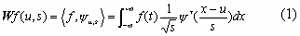
The continuous wavelet transform (CWT) which decomposes signals over dilated and translated wavelets was first introduced by Grossmann and Morlet (1984). The wavelet transform of a function ¦Î L ²(R) is defined by

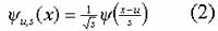
where y_u,s(x) is obtained by introducing a scale factor s and a translation factor u to the mother wavelet function y(x) :

The wavelet transform W¦(u,s) is a function of the scale and the spatial position x. It measures the variation in ¦ in the neighborhood of u, whose size is proportional to s. When the scale s varies from its maximum to zero, the decay of the wavelet coefficients characterizes the regularity of ¦ in the neighborhood of u. This is the essential idea in detecting the absorption band position from the reflectance spectra.

3.2 Modulus Maxima of Wavelet Transform
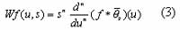
A wavelet y with n vanishing moments can be written as the n^th order derivative of a function q , that is y=(-1)ⁿ q⁽ⁿ⁾ , thus the resulting wavelet transform is a multiscale differential operator:

Suppose the convolution

averages f(x) over a domain proportional to s. Let y₁=-q' and y₂=q'' be two wavelets, thus the wavelet transforms, W¹¦(u,s) and W²¦(u,s), are respective to the first and second derivative of ¦(x) smoothed by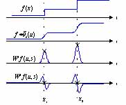

Figure 1. The positions of the local maxima of and the zero-crossing of

. For a fixed scale, the local maxima of W¹¦(u,s) and the zero-crossings of W¦(u,s) will correspond to the inflection points of

(figure 1). For all scales, the local maxima points of W¹¦(u,s) can be connected as a set of maximal lines in the scale-space plane (u, s). Similarly, the zero-crossings of W²¦(u,s) define a set of smooth curves that often look like fingerprints. By detecting the positions of the local maxima or zero-crossings from a coarse to fine scale, we can obtain the positions of the singularities of a signal. These two methods are very similar, but the local maxima approach has several important advantages (Mallat and Hwang, 1992). The smoothing function q can be viewed as the impulse response of a low-pass filter. An important example often used in signal processing is the Gaussian function. In this study, the wavelet is defined as the first derivative of the Gaussian function.

3.3 The Estimation of Lipschitz Regularity

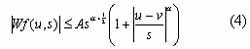
To characterize the singular structure of a signal, it is necessary to quantify local regularities precisely. Lipschitz exponents provide not only uniform regularity measurements over time intervals, but also pointwise Lipschitz regularity at any point v of a signal. The relationship between the decay of the wavelet transform amplitude across scales and the pointwise Lipschitz regularity of the signal was described by Jaffard (1991). He proved a necessary and sufficient condition in the wavelet transform for estimating the Lipschitz regularity of ¦ at a point v. Assume that the wavelet y has n vanishing moments and n derivatives with a fast decay. If ¦Î L²(R) is Lipschitz a£n at v, then there exists A>0 such that "(u,s)Î Rx R⁺ ,

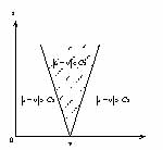
In order to simplify the above condition, we assume that y has a compact support equal to [-C,C] . The cone of influence of v in the scale-space plane is the set of points (u, s) such that v is included in the support of

(Mallat, 1997). Since the support of

is equal to [u-Cs,u+Cs], the cone of influence of v is defined by½u-v½£Cs . This is illustrated in Figure 2. Since ½u-v½£Cs, the conditions (4) and (5) can be written as

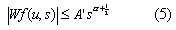
which is equivalent to the uniform Lipschitz condition given by Mallat (1997). In this study, we assumed that all modulus maxima converging to v are included in a cone. The potential singularity at v is isolated. Function ¦ is uniformly Lipschitz a in the neighborhood of v if and only if there exist A>0 such that each modulus maximum (u, s) in the cone satisfies (6). In order to estimate the Lipschitz exponent we rewrite (5) as

.The Lipschitz regularity at v is thus the maximum slope of log₂½W¦(u,s)½ as a function of log₂s along the maxima lines converging to v.

4. Experiments

4.1 Test data
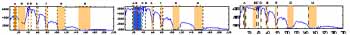
The test data are a set of hyperspectral data delivered from AVIRIS. The data has 220 spectral bands from 0.4um to 2.5um with about 10 nm spectral resolution. The spectral curves of three different materials are shown in Figure3.

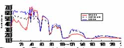
Figure 3. Three kinds of hyperspectral curves from AVIRIS images.

(a) grass (b) soybean (c) corn
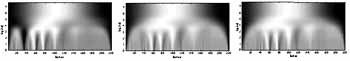
Figure 4. W¦(u,s), wavelet transform of the spectrums,

(a) grass (b) soybean (c) corn
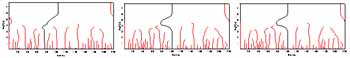
Figure 5. The modulus maxima of W¦(u,s)

(a) grass (b) soybean (c) corn
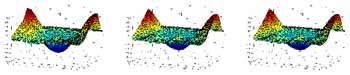
Figure 6. 3D view ofW¦(u,s)

(a) grass (b) soybean (c) corn
Figure 7. The spectral features extracted by modulus maxima of
W¦(u,s)

4.2 Wavelet Transform Modulus
Figures 4(a), (b) and (c) show the wavelet transform of the spectral curves with respect to the three materials. They were calculated with , where is a Gaussian function. The position parameter u and the log2 of scale s vary respectively along the horizontal and vertical axes. Black, gray and white points represent positive, zero and negative wavelet coefficients respectively. Figures 5(a), (b) and (c) show the results of extracting modulus maxima from . It can be seen that all singularities can be detected easily along the maxima line from coarse to fine scales. The maxima lines detected along the scale space correspond to the main absorption bands of the spectral curve. The 3D views of the wavelet transform are respectively shown in figures 6(a), (b) and (c). The absorption bands create large amplitude coefficients in their cone of influence. In figure 7(a), (b) and (c), eight absorption spectral features are marked with gray rectangles A… E. The left and right borders of the rectangles are determined by the maxima lines. The converged position of a maxima line with negative wavelet coefficients correspond to the left border of a rectangle, then the right border of the rectangle will be determined by the next maxima line with positive wavelet coefficients. Because the spectral curves of these three materials are very similar in shape, the extracted spectral features C, D, E, F, and G almost have the same positions (See table 1.). However, these three materials can be differentiated using the features A, B, and H, which are represent small variations of the spectral curves.

4.3 Lipschitz Exponent
Figure 8 shows the results of Lipschitz exponents calculated at each singularity point for the test data. Because the Lipschitz regular was estimated under the assumption of the compact support wavelet with one vanishing moment, the values of should satisfy for isolated singularity. The negative Lipschitz exponent values indicate the corresponding points possessing high-frequency oscillations in their neighborhood.

The spectral curves for soybean and corn shown in figure 5 look quite similar in shape and their main absorption bands corresponding to the low-frequency components are nearly the same. However, one would easily discover the differences when a scale factor is introduced to overlap these two curves. Figure 9 obviously shows that the high-frequency variations in the corn spectrum are larger than the soybean spectrum in the 21st, 76th and 153rd bands. Therefore, these two different materials can be distinguished easily with the Lipschitz exponents. Table 1. shows that the spectral features C, D, E, F, and G have the same positions in spectral curves, but their Lipschitz exponents are different. The variations will be useful to distinguish a spectral curve. For example, the grass spectral curve at the right boder of E feature is smoother than the other two curves at the same location, so its Lipschitz exponent is larger than the other two.

Table1. Results of spectral absorption positions

Absorption features		A		B		C		D		E		F		G		H
Parameters		L	R	L	R	L	R	L	R	L	R	L	R	L	R	L	R
Grass	Band	9	14	18	36	39	41	45	47	57	61	76	81	101	118	146	172
Grass	Lips. exp.	0.756	-0.174	0.669	0.777	-2.800	-1.283	0.116	-0.350	0.618	0.555	0.752	0.281	0.826	0.852	0.898	0.854
Soybean	Band	18	37	23	29	39	41	45	47	57	61	76	81	102	117	147	166
Soybean	Lips. exp.	0.614	0.116	0.670	0.251	-1.894	-1.286	-0.122	0.079	0.710	0.560	0.911	0.320	0.909	0.553	0.760	0.492
Corn	Band	9	14	29	37	39	41	45	47	57	61	76	81	102	117	147	166
Corn	Lips. exp.	-0.106	-0.319	0.411	-0.17	-1.71	-1.300	0.255	-0.216	0.857	0.553	0.400	0.293	0.827	0.547	0.805	0.571

5. Discussion
The high spectral resolution of hyperspectral data provides the ability for diagnostic identification of various materials. In order to increase the classification performance, feature extraction is pre-processed to substantially remove the redundant information without sacrificing significant information. In this study, we transferred the hyperspectral data into the scale-space plane using the wavelet transform to extract important spectral features. The wavelet transform can focus on localized signal structures by scaling and dilating a wavelet. The absorption bands of spectral curves are thus detected automatically by the wavelet transform modulus maxima, and the Lipschitz exponents are estimated at each singularity point in the spectral curve from the decay of the wavelet transform amplitude. The local frequency variances provide useful information about the oscillations in the hyperspectral curve for each pixel. Various materials can be distinguished by the differences in the local frequency variations. This new method generates features that are more meaningful and is more stable than other known methods for spectral feature extraction. In particular, the method proposed in this paper will be helpful for spectral analysis that reduces the multidimensional hyperspectral data to a smaller number of essential features that can be both automatically processed and physically interpreted.

Acknowledgements
The authors would like to thank the National Science Council of Republic of China, for support of this research project: NSC88-2211-E006-084.

Reference

Demetriades-Shah, T.H., M.D. Steven and J.A. Clark, 1990. High Resolution Derivatives Spectra in Remote Sensing. Remote Sens. Environ, 33, pp. 55-64.
Grossmann, A. and J. Morlet, 1984. .Decomposition of Hardy functions into square integrable wavelets of constant shape. SIAM J. Math, 5 , pp.723-736.
Hsu, P.H. and Y.H. Tseng, 1999. Feature Extraction for Hyperspectral Image. Proceedings of the 20th Asian Conference on Remote Sensing, Vol. 1, pp. 405-410.
Hughes, G.F., 1968. On the Mean Accuracy of Statistical Pattern Recognizers. IEEE Transaction on Information Theory, IT-14, pp. 55-63
Jaffard, S., 1991. Pointwise smoothness, two microlocalisation and wavelet coefficients. Publications Mathematiques, 35.
Lee, C. and D. Landgrebe, 1993. Feature Extraction and Classification Algorithms for High Dimensional Data. TR-EE 93-1, Purdue University.
Lillesand, T.M. and R.W. Kiffer, 2000. Remote Sensing and Image Interpretation, Fourth Edition, John Wiley & Sons, Inc.
Mallat, S. and W. L. Hwang, 1992. Singularity Detection and Processing with Wavelets. IEEE Transactions on Information Theory, 38(2), pp. 617-643.
Mallat, S., 1997. A wavelet tour of signal processing, ACADEMIC PRESS.
Philpot, W.D., 1991. The Derivative Ratio Algorithm: Avoiding Atmospheric Effects in Remote Sensing. IEEE Transactions on Geoscience and Remote Sensing, 29(3), pp.350-357.
Piech, M.A. and K.R. Piech, 1987. Symbolic representation of hyperspectral data. Applied Optic, 26(18), pp. 4018-4026.
Piech, M.A. and K. R. Piech, 1989. Hyperspectral interactions: invariance and scaling. Applied Optic, 28(3), pp.481-489.
Richards, J.A., 1993. Remote Sensing Digital Image Analysis: An Introduction. Springer-Verlag Berlin Heidelberg, Second Edition.
Schowengerdt, R.A., 1997. Remote Sensing: Models and Methods for Image Processing, Academic Press.
Tadjudin, S. and D. Landgrebe, 1998. Classification of High Dimensional Data with Limited Training Samples. PhD Thesis and School of Electrical & Computer Engineering Technical Report TR-ECE 98-8, Purdue University.
Tsai, F. and W. Philpot, 1997. Derivative Analysis of Hyperspectral Data for Detecting Spectral Features. IGARSS '97, Remote Sensing - A Scientific Vision for Sustainable Development,Vol.3, pp.1243-1245.
Tsai, F. and W. Philpot, 1998. Derivative Analysis of Hyperspectral Data. Remote Sens. Environ, 66, pp.41-51.