| GISdevelopment.net ---> AARS ---> ACRS 2000 ---> Hyperspectral & Data Acquisition Systems |
Vegetation Spectral Feature
Extraction Model
Qian Tan , Hui
Lin
Dept. of Geography & Joint Lab. For Geoinformation Science ,
The Chinese University of Hong Kong , Hong Kong
Tel: (+852)-26098105
E-mail: tanqian@cuhk.edu.hk
Yongchao Zhao , Tong Qingxi , Zhen Lanfeng
Lab. Of Remote sensing Information Sciences ,
Institute of Remote Sensing Applications ,CAS ,
Beijing , 100101 , China
Keywords:vegetation, hyperspectral, spectral
feature extraction Dept. of Geography & Joint Lab. For Geoinformation Science ,
The Chinese University of Hong Kong , Hong Kong
Tel: (+852)-26098105
E-mail: tanqian@cuhk.edu.hk
Yongchao Zhao , Tong Qingxi , Zhen Lanfeng
Lab. Of Remote sensing Information Sciences ,
Institute of Remote Sensing Applications ,CAS ,
Beijing , 100101 , China
Abstract
A new spectral feature selection and extraction model(for vegetation only!)--- Vegetation Spectral Feature Extraction Model (VSFEM) is presented . A lot of vegetation field spectrum analyzed , 8 vegetation spectral feature positions are acquired , through which a series of feature parameters are achieved .
1. Introduction
Spectral feature extraction were mostly from or for target classification .
Principle Component Analysis (PCA) is used by most people . This method produces a new series of images , put in order by information content (or variance ) . Relationships among images are essentially removed . With forward principle components , most information content can be seen , which is the optimal result for minimum mean square error . Green (1988) developed PCA , who applied MNF (Minimum Noise Fraction) so as to make every component after MNF transform in order by signal-to-noise ratio (S/N) from large to small , instead of variance . Jia (1999) developed PCA to segment PCA to make feature extraction , whose classification and display result has made some progress . Though PCA can compress and extract information with minimum mean square error , information of principle component images is hard to explain directly according to spectrum , moreover , sample distribution not considered , it's uncertain to get optimal classification result . After realizing this problem , Fukunaga (1970) proposed a new transform method , that was , to find an transform matrix , who satisfied the formula , T(S1+S2)T-T=I , in which Si is the correlation matrix of class i . This method is effective when differences of average values are small and covariance play a key role , but for common situation , is ineffective (Foley , 1975) . Kazakos (1978) put forward a feature extraction algorithm ---linear scalar extraction , making minimum classification error probability for two classes of multi-dimension normal distribution . This method can find an optimal vector to get minimum classification error probability , but when more than one feature is required , this method has no power . After considering within-class and between-class distance , Richard (1986 ) posed a feature extraction method---Canonical Analysis (CA) , Lee (1993) raised a feature extraction method based on decision boundary .
This paper puts forward VSFEM(Vegetation Spectral Feature Extraction Model) , which is very different from above methods . VSFEM aims at vegetation spectral feature extraction , from or for controlling vegetation spectral curves , through an amount of analysis of field vegetation spectral curves to get some regularity . Compared to above methods , VSFEM pay much attention to target spectral reflection of biological and physical features , not thinking feature extraction just as pattern recognition or information compression of a branch of mathmatics .
2. Study Area and Data Collection
Study Area
A study area near Changzhou city, Jiangsu Province, China was chosen for collecting ground data . The study focused on vegetation , which included principle types of agricultural crops and trees in the study area , such as , rice , maize , peanut , sweet potato , cotton ,soybean , cabbage , carrot , etc .
Data Collection
During the period from late August(middle season in vegetation growing circle) to mid-October(later season in vegetation growing circle), 55 field vegetation spectral data were acquired from 20 sites in Changzhou by SE-590 ---a portable field spectroradiometer . At the same time , some biochemical parameters , such as chlorophll concentration , leaf area index(LAI) were measured . Data were collected in nadir orientation of the radiometer and at about 45° solar zenith angle. Four scans at a time were averaged as the final spectra in each measurement. In addition , the data were collected from 11:00 to 13:00 .
When trees were measured , branches with leaves were picked down and laid on the ground. The specific parameters of SE-590 Portable Field Spectroradiometer are shown as follows:
Wavelength: 400 - 1100 nm
Spectral resolution : 4.0 nm
Sample channels: 252
Field of view:150
3. Methodology
3.1 Vegetation Spectral Feature Extraction Model
There are some special features, such as "green peak", "red valley" and "NIR platform", in the curve of the reflectance, reflectance intensities of these featured positions vary remarkably or regularly with the species or growth periods. So, it is possible that we design special parameters that are good tokens of curve shape of different species or growth stages. Moreover , if we want to discuss correlation between spectra and vegetation biochemical properties, we also need to find some special spectral parameters. For this case, we define eight special positions(feature position) and design many parameters(feature parameter) like NDVI to discuss the species and property(including the growth stage) difference of typical vegetation in Changzhou. All the eight feature positions as M, B, G, Y, R, V, I1 and I, and some feature parameters are shown in fig.1 . This figure shows a typical spectral curve R(l) .The definition of 8 feature positions as shown in fig.1 and their agorithms are as follows:
- Absorption peak in purple-blue band-M(lM,RM): The position where the
reflectance is the minimum in the wavelength range of
<500nm:
RM=MIN(R(lÎ380-500nm)),lM,li(R(li)=RM) - Absorption edge of blue waveband (blue edge)-B(lB,RB): the turning point of
the spectral curve in the range of 500-550nm, defined as the maximum
point in the first-order derivative value in the same waveband region:
lB=li(R'(l)=MAX(R'(lÎ450-550nm)),RB=R(lB) - Reflectance peak of green band(green peak)-G(lG,RG): the maximum position of reflectance band from 500-600 as: RG=MAX(R(lÎ500-600nm)),lG=li(R(li)=RG)
- Absorption edge of yellow waveband(yellow edge)-Y(lY,RY): the turning point of
the spectral curve in the range of 550-650nm, defined as the minimum
point in the first-order derivative in this range:
lY=li(R'(l)=MIN(R'(lÎ550-650nm)),RY=R(lY) - Absorption peak in red band(red "valley")-R(lR,RR): where the reflectance
is the minimum in the red band of 600-720nm:
RR=MIN(R(lÎ600-720nm)),lR=li(R(li)=RR) - Red edge-V(lV,RV):
the turning point of reflectance curve within waveband of red-NIR, the
maximum point of the first-order derivative spectral curve in 670-780nm:
lV=li(R ' (l)=MAX(R '(lÎ670-780nm)) , RV=R(lV) - Start site of the NIR platform-I1(lI1 , RI1): the transition
point between the red slope in wavelength >760nm and the NIR
platform. It is also defined as the first joining point of the spectral
curve and its continuum curve in range of 670-800nm as shown in fig
5.4.A. Its arithmetic is:
lI1=li(Rcr(lÎ670-800nm)) , RI1=R(lI1) - Maximum point of reflectance in NIR of 780-950-I(lI , RI):
RI=MAX(R(lÎ780-950nm)) , lI=li(R(li)=RI)
lG'= l(R'(lÎ500-600nm)=0)
lR'=l(R'( lÎ600-720nm)=0)

Fig 1. sketch of 8 feature positions and some feature parameters for the green vegetation in Changzhou
The reflectance is about Rice measured in Aug. 31 at Changzhou. The parameters and positions labeled in this sketch are defined in the text.
As shown in fig.1, the eight special positions determine, on the whole, shape and spectral feature of reflectance spectra of vegetation in visible-near infrared band. It is distinct that the multi-line MBGYR determines the feature of green peak while the multi-line GYRVI1 determines the general shape of red absorption peak. Line I1I can be looked upon as the representation of NIR platform. As shown in Table 1 , these 8 positions almost keep constant with outer changes while their corresponding reflectivity intensities vary greatly .Thus there is some possibility that we can use a variety of these 8 special positions and their relations to represent spectral change of different vegetation.
In order to figure out the correlative variety of these special position and therefore to show the changing rules of reflectance spectra with vegetation species, we designed some parameters(feature parameters) on the base of the 8 special positions according to the spectral features in fig 1. They are:
- The coordinate of 8 feature position M, B, G, Y, R, V, I1, I and two accessorial positions as G' and R': (lP , RP). where the subscript P is the name of these positions, l is the wavelength and R is the reflectance. Obviously, there have 20 such parameters and in general we have G' » G and R' » R.
- Slope of blue edge-SB: the slope of line
MG.
SB=(RG-RM)/(lG-lM)
Thus it approximately determines the curve of MBG. - Slope of yellow edge-SY: the slope of line RG. It
approximately determines the character of curve GYR:
SB=(RG-RR)/(lG-lR) - Slope of the incline among bands of red-NIR-SV:: the
slope of line RI1 , it is a representation of curve
RVI1:
SV=(RI1-RR)/(lI1-lR) - Slope of the continuum-SC: the slope of line
GI1. It generally reflects the background feature of the
absorption peak GYRVI1:
SC=(RG-RI1)/(lG-lI1) - Net height of green peak-HG: the distance between G and
line MR in the dimension of reflectance. It generally equals to the net
reflectance of the background-removed green peak and is the reflection
of reflectance peak MBGYR:
HG=RG-((RR-RM)/(lR-lM)×(lG-lR)+RR) - Net depth of red absorption "valley"-HR: the distance
between R and line GI1 in the dimension of reflectance. It's
can be looked upon as background-removed depth of red absorption peak
and reflects the feature of peak GYRVI1:
HR=(RG-RI1)/(lG-lI1)×(lR-lG)+RG-RR - Net height of infrared platform-HI: the difference
between the averaged reflectance of NIR platform and the reflectance of
point R. It can be substituted by the reflectance difference of R and
the midpoint of line I1I and reflects the feature of platform
I1I:
HI=(å((Ri+Ri+1)×(li+1-li)/2))/Dl-RR»(RI1+RI)/2-RR,
where liÎlI1-930nm, Dl is the width of NIR=930-lI1. - FWFH of green peak-lwG:
generally represents the width of green peak. It is approximately
calculated as the horizontal interval between points B and Y:
lwG »lY-lB - FWFH of red absorption peak-lwR:
the reflection of the width of red "valley". It is calculated as the
half width of continuum-removed red "valley" and can be replaced as the
horizontal interval of line YV:
lwR»lV-lB - Averaged reflectance of NIR platform-RIa: can be
substituted by the reflectance average of I1 and I:
RIa=(å((Ri+Ri+1)×(li+1-li)/2))/Dl»(RI1+RI)/2=HI+RR
where liÎlI1-930nm, Dl is the width as 930-lI1. - Area of green peak-AG: the integrated area under curve
MBGYR. It is the embodiment of green peak intensity and can be
approximately substituted by the area under multiline MBGYR:
AG=(å((Ri+Ri+1)×(li+1-li)/2))
»[(å(Rp+Rp+1)×(lp+1-lp)/2)),p=M,B,G,Y]
where liÎlM-lR. - Pure area of green peak-AG': the integrated area
enveloped by curve MBGYR and line MR. It is the net intensity of green
peak and obviously can be replaced by the area of polygon MBGYRM:
AG'=AG-((RM+RR)×(lR-lM)/2)
»[(å(Rp+Rp+1)×(lp+1-lp)/2)],p=M,B,G,Y]
-((RM+RR)×(lR-lM)/2)
where liÎlM-lR - Net area of red absorption peak-AR: the area enclosed by
curve GYRVI1 and line GI1. It can estimate as the
area of polygon GYRVI1G:
AR=SGYRVI1G
It should be pointed out that the usually applied parameters in vegetation study such as NDVI, red edge lre and red edge slope drre could also be obtained from these parameters as follows:
NDVI=(RI1-RR)/(RI1+RR) , lre=lV , drre»SV
Therefore, the definition of eight feature positions not only reflects the general feature of the reflectance data, but also can get many high-information-content feature parameters that may have good relationships with some property parameters of vegetation such as chlorophyll concentration.
3.2 Analysis for Effectiveness of VSFEM---Relative Stability of Position
To study characteristics of the above feature positions and parameters , especially to study relationships between feature positions and vegetation types , as well as action of feature parameters for reflecting vegetation parameters . Based on above definitions and algorithms , more than 100 spectral data of about 20 types of vegetation in Chang Zhou were analyzed to get spectral feature positions and parameters.
Table 1 gives principle results , from which we can see that ,
under the research conditions of the experiment , all feature positions , especially 8 feature positions are stable , these positions are : M:404, B:525, G:556,Y:573,R:671,V:723,I1:758,I :900nm, take I position as example , which has the largest change range , for 62 samples at different time and place , its confidence width is 6.4nm , others less than 3nm , even for standard deviation , are less than 6nm generally . This kind of confidence interval has been super than spectral resolution of many instruments .
| Feature position | samples | average(nm) | Standard deviation | Relative error(%) | 95%confidence(nm) | Range of 95%confidence(nm) | Width of 95%confidence(nm) |
| lB | 62 | 524.7 | 1.04 | 0.20 | 0.3 | 524.5 - 525.0 | 0.5 |
| lG | 62 | 556.2 | 3.67 | 0.66 | 0.9 | 555.3 - 557.1 | 1.8 |
| lI | 62 | 900.7 | 12.77 | 1.42 | 3.2 | 897.5 - 903.8 | 6.4 |
| lI1 | 62 | 758.3 | 7.01 | 0.92 | 1.7 | 756.5 - 760.0 | 3.5 |
| lM | 62 | 403.9 | 2.72 | 0.67 | 0.7 | 403.3 - 404.6 | 1.4 |
| lR | 62 | 671.4 | 2.40 | 0.36 | 0.6 | 670.8 - 672.0 | 1.2 |
| lV | 62 | 723.4 | 9.80 | 1.35 | 2.4 | 720.9 - 725.8 | 4.9 |
| lY | 59 | 573.2 | 0.81 | 0.14 | 0.2 | 572.9 - 573.4 | 0.4 |
3.3 Rediscussion for VSFEM---Reduction of Some Feature Positions
In addition , we calculate the correlation coefficients between different bands for all the spectral vegetation data measured by Se590 to show the independence of the bands and to select the most information-containing band group in order to indicate more efficiently the difference among different vegetation species , through which we can prove the effectiveness of VSFEM
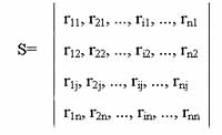
where S is the correlation coefficient matrix of all bands, rij is the absolute value of correlation coefficient between band i and band j. Obviously:
rij=rji=|Lij/SQRT(Liix Ljj)|
where Lij is the covariance between band i and band j.
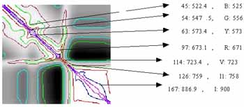
Fig. 2 is the simulated image of the correlation coefficient matrix among 187 bands that is calculated on the base of 71 vegetation . Curves in Fig. 2 are isolines , from diagonal line to outside , the values are 0.9999,0.999,0.99,0.95,0.9,0.5,0.3 and 0.1 in the order .
From Fig. 2 we can see that ,
Except band 100(band number of Se590) to 126 , for vegetation , correlation coefficient are all very high (more than 99.99% generally) , that is to say, it's practical for band reduction .It shows two high-correlative platforms of 400-670nm and 760-950nm respectively, which means within these two regions , a few bands are enough to extract vegetation information . Moreover , around 550nm and 670nm , there are relatively wider areas . It's unnecessary to subdivide bands in these regions . but between 675nm---775nm and around 522nm and around 573nm , correlation coefficient are low generally . This shows more information here and bands should be subdivided . compared to 8 feature positions referred before , we can get that , for vegetation research , those regions that should be subdivided are just blue edge B , yellow edge Y and red edge V, while those regions that needn't be subdivided are blue absorption valley M , green peak G , red absorption valley R , and NIR platform I . In Fig. 2 , position B , Y and V are located in the center of narrow regions of isolines , while M , G , R , I in the center of broad regions . The arrows in Fig. 2 explain this clearly .
Table 2 lists correlation matrix of 8 feature positions , from Table 2 , we can get priority order for 8 feature positions : first , select two positions with minimum correlation coefficient (absolute value) , remove these two bands and those bands with highest correlation coefficient with them , then , select repeatedly for the rest bands until we get to band number we predetermine.
| Corresponding feature position | M | B | G | Y | R | V | I1 | I |
| Wavelength(nm) | 404.7 | 522.4 | 544.7 | 573.4 | 673.1 | 723.4 | 759.0 | 890.1 |
| 404.7 | 0.8890 | 0.8952 | 0.8372 | 0.4575 | 0.8408 | 0.6561 | 0.6117 | |
| 522.4 | 0.8890 | 0.9895 | 0.9925 | 0.7071 | 0.8265 | 0.5520 | 0.5185 | |
| 544.7 | 0.8952 | 0.9895 | 0.9812 | 0.6161 | 0.8785 | 0.6364 | 0.6035 | |
| 573.4 | 0.8372 | 0.9925 | 0.9812 | 0.7455 | 0.7960 | 0.5053 | 0.4758 | |
| 673.1 | 0.4575 | 0.7071 | 0.6161 | 0.7455 | 0.3313 | -0.0230 | -0.0366 | |
| 723.4 | 0.8408 | 0.8265 | 0.8785 | 0.7960 | 0.3313 | 0.9020 | 0.8806 | |
| 759.0 | 0.6561 | 0.5520 | 0.6364 | 0.5053 | -0.0230 | 0.9020 | 0.9947 | |
| 890.1 | 0.6117 | 0.5185 | 0.6035 | 0.4758 | -0.0366 | 0.8806 | 0.9947 |
Fig. 2 The simulated images of the correlation coefficient matrix among 187 bands(400-950nm) of Se590
from Table 2 , we can get priority order for 8 feature positions : first , select two positions with minimum correlation coefficient (absolute value) , remove these two bands and those bands with highest correlation coefficient with them , then , select repeatedly for the rest bands until we get to band number we predetermine.
4. Conclusion
According to above analysis , we find out that:
- Through lots of analysis on field vegetation spectral data, A new spectral feature selection and extraction model(for vegetation only!)--- Vegetation Spectral Feature Extraction Model (VSFEM) is presented , with which 8 spectral feature positions are suggested to control vegetation spectral curves . Those feature positions are 404(M), 525(B), 556(G),573(Y),671(R),723(V),758(I1),900nm(I) .
- It is reasonable to select feature positions as best bands. However, the feature positions and bandwidths for different feature are not the same. As a result, the accurate positions of G, R, M, I are not necessary. They should change in a proper range, such as I and M which could use a broader band.
- According to the correlationship among bands, the bands could be removed are: I, M, B, Y and G. As for band R ¢ V ¢ I1, they should not be removed . If subdivision allowed , it's proper to subdivide red edge(R-V-I1 ) , moreover , we can subdivide around B and Y position .
References
- Boardman, J. W., and Kruse, F. A., 1994,"Automated spectral analysis: a geological example using AVIRIS data, north Grapevine Mountains, Nevada.", Proceedings, ERIM Tenth Thematic Conference on Geologic Remote Sensing, Environmental Research Institute of Michigan, Ann Arbor, MI, p. I-407 - I-418.
- Fukunaga,K., Koontz,W.L.G., 1970, "Application of the Karhunen_Loeve expansion to feature selection and ordering." , IEEE Trans. Comput., Vol. C-19,No.4,pp311-318,Apr.1970.
- Green, A. A., Berman, M., Switzer, P, and Craig, M. D., 1988, "A transformation for ordering multispectral data in terms of image quality with implications for noise removal", IEEE Transactions on Geoscience and Remote Sensing, v. 26, no. 1, p. 65-74.
- Jia,Xiuping, Richards,J. A.,1999, "Segmented principal components transformation for efficient hyperspectral remote-sensing image display and classification.", IEEE Trans. On Geosci. And Remote Sensing, Vol.37, No.1, 538-542, Jan. 1999.
- Kazakos,D.,1978, "On the optimal linear feature." , IEEE Trans. Inform. Theory, Vol. IT-24,No.5,pp651-652,Sept. 1978.
- Lee, C. and Landgrebe, D. A.,1993, "Feature extraction based on decision boundaries.", IEEE Trans on P.A.M.I. Vol. 15, No.4, April 1993.
- Richards,John A., Remote Sensing Digital Image Analysis, An Introduction, Spriger-Verlag,1986.
The authors wish to thank Laboratory of Remote Sensing Information Sciences , Institute of Remote Sensing Applications for providing the data and their sincere help .