| GISdevelopment.net ---> AARS ---> ACRS 2000 ---> GIS & Data Integration |
Implementation of A
Geographic Information System (GIS) to Determine Wildlife Habitat Quality
Using Habitat Suitability Index
YuChing Lai
Post Doctor, Division of Forest Management
Taiwan Forestry Research Institute
53 Nan-Hai Road, Taipei 100, TAIWAN
Walter L. Mills
Associate Professor of Forestry,
Department of Forestry and Natural Resource
Purdue University, 1159 Forestry Building, Room 110
West Lafayette, IN 47907-1159
Chi-Chuan Cheng
Deputy Director, Taiwan Forestry Research Institute
Council of Agriculture, 53 Nanhai Rd., Taipei 100,TAIWAN
Key Words: Geographic Information System (GIS), Habitat Suitability Index (HSI), Wildlife Habitat, Spatial Pattern
Abstract : Habitat quality for many wildlife populations has a spatial component related to the arrangement of habitat elements across large geographic areas. There are a number of indices used to quantitatively describe the components of habitat assessment, yet, only a few of them incorporating spatial relationship in the model. Among these mathematical indices, habitat Suitability Index (HSI) models have been widely developed for use in habitat evaluation procedures (HEP). HEP, which is based on the assumption that habitat for a selected wildlife species can be described by a Habitat Suitability Index, can be used to document the quality and quantity of available habitat for a specific wildlife species. However, because of the difficult of quantifying spatial arrangement, HSI has ignored the spatial distribution of habitats. Geographic information system (GIS) provides wildlife managers and planners with techniques that can help overcome some of the problems inherent in developing, applying, and evaluating practical, spatially explicit habitat models. Given the desirability of deterministic results, seamless integration of data and analytical options available via GIS increases our ability to state, implement, test, and evaluate estimated or modeled habitat elements. This study examined possible ways to use the accumulated knowledge found in HSI to estimate the wildlife microhabitat quality across a landscape. In this study, GIS is used to generate parameters of HSI models, especially the spatial habitat parameters that are often of explicit importance for HSI models, incorporating spatial reasoning and constraints into HSI models, analyzing spatial patterns of habitat, and providing the mapping capability for converting stand-based information into maps of habitat. Species that occur in Missouri Ozark Forest Ecosystem with existing HSI models are selected. A moving window the size of the home ranges of each species is applied to calculate the average value of each life requisites. In conclusion, implementing GIS in wildlife habitat assessment improves the use of HSI models by automating tasks, identifying areas where site-specific analyses were needed, and reducing the spatial and temporal complexity involved with integrating different resource perspectives.
1. Introduction
Ecosystem management appears to be the wave of the future. General program goals such as "maintain biodiversity", "maintain viable populations of all native species", and "protect representative natural communities" are often emphasized in ecosystem management (USDA 1994, Grumbine 1994, and Irland 1994). Tools for maintaining biodiversity and viable species populations are likely to be focused on providing habitats in an appropriate spatial and temporal arrangement. Therefore, vegetation management is a major tool for maintaining and restoring biodiversity and to achieve delisting or to avoid listing of threatened and endangered species (USDA 1994). There have been numerous attempts to assess habitat quality for particular species. Probably the most widely practiced in the United States is the Habitat Suitability Index (HSI), which together with the Habitat Evaluation Procedures (HEP) developed by the U.S. Fish and Wildlife Service, has frequently been used to assess habitat. It is also a useful monitoring tool for biodiversity at community-ecosystem level (Noss and Cooperrider 1994). However, it ignores the effects of immigration and spatial distribution of habitats (Carroll and Meffe 1994). In this study, the possibility of using HSI for ecosystem management assessment will be tested. Species with existing HSI models will be use. Since the same procedure can be applied regardless of what species is used, more species could be used when, and if, appropriate HSI are developed. Point sample data combined with spatial data of the Missouri Ozark Forest Ecosystem Project (MOFEP) will be used to assess ecological organization at the community-ecosystem level in this study.
2. Methodology
Study Area
The Missouri Ozark Forest was located in southeastern Missouri Ozarks consists of 9,200 acres of mature upland oak-hickory and oak-pine forest communities. Collectively, these counties are 84% forested with large contiguous blocks of forests separated only by roads and streams. Compartment One of Missouri Ozark Forest Ecosystem Project (MOFEP) was selected for this study because it has the most detailed inventory data. It is 380 hectares (989 acres) in size and contained 62 stands. Seventy-six permanent sample plots are distributed among these stands. Dominant overstory species included pine (Pinus echinata), hickory , and oak. A cluster plot design was used to collect data in order to investigate the effects of forest management on the composition and spatial distribution of woody and herbaceous vegetation. In this design, a 0.2 ha (0.49 ac.) circular plot was used to sample trees 11.4 cm (4.5 in) dbh and larger and to tally the total number of den trees. Four line intercepted 17.2 m (56.4 feet) in length were located within each 0.2 ha plot to measure the coverage of down dead woody material. Four circular 0.02 ha (0.05 ac.) plots were located within the larger plot to sample woody plants between 3.5 cm (1.5 in.) and 11.2 cm (4.4 in.) dbh. One 0.004 ha (0.01 ac) plot was placed within each 0.02 ha plot, sharing the same plot center, to sample vegetation taller than 1.0 m (3.3 feet) and less than 3.5 cm (1.5 inches) dbh. Four one square m (10.8 square feet) plots were located within each 0.02 ha plot to sample vegetation less than 1.0 m (3.3 feet) in height.
2.2 HSI Models selection
While hundreds of habitat suitability index models were available, the selected HSI represent those that were valid for the Missouri Ozark Highland and for which data was available. Eleven species were selected for this study including seven bird species and four mammals. The bird species were selected when either their breeding range or year-round range include the Missouri Ozark highland. They were barred owl (Strix varia) (Allen 1987), brown thrasher (Toxostoma rufum) (Cade 1986), downy woodpecker (Picoides pubescens) (Schroeder 1982), hairy woodpecker (Picoides villosus) (Sousa 1987), pileated woodpecker (Dryocopus pileatus) (Schroeder 1982), eastern wild turkey (Meleagris gallopavo sylvestris) (Schroeder 1985), and northern bobwhite (Colinus virginianus) (Schroeder 1985). Four mammal HSI models were selected, i.e., Bobcat (Felis rufus) (Boyle and Fendley 1987, Schwartz and Schwartz 1981), eastern cottontail (Sylvilagus floridanus) (Allen 1984, Schwartz and Schwartz 1981), gray squirrel (Sciurus carolinensis) (Allen 1982, Schwartz and Schwartz 1981), and fox squirrel (Sciurus niger) (Allen 1982, Schwartz and Schwartz 1981). In most of these wildlife HSI models, more than one life requisite (for example, food, cover, and reproduction) was usually used (Table 1). Each of the life requisite was described by a set of habitat variables (Table 1).
|
Attributes Species |
Home Range(ha) | Life Requisities | Variables |
| BARRED OWL | 228.6 | Reproduction | # of trees >51 cm dbh, mean dbh, Canopy cover |
| BOBCAT | 100 | Food | % by grass/forb-shrub |
| BROWN THRASHER | 1 | Food/cover/reproduction | Density, Canopy cover, Litter cover |
| DOWNY WOODPECKER | 4 | Food/reproduction | Basal area,# of snags >15cm dbh |
| EASTERN COTTONTAIL | 4 | Cover/ | Herbaceous cover, Shrub cover, Canopy cover |
| FOX SQUIRREL | 3.55 | Food/cover | Canopy closure of hard mast trees,
Distance to grain, mean dbh canopy cover, shrub cover |
| GRAY SQUIRREL | 0.4 | Food/cover | Canopy closure of mast trees, Distance of hard mast trees, canopy cover, mean dbh, shrub cover |
| HAIRY WOODPECKER | 4 | Cover/reproduction | Mean dbh, Canopy cover, Canopy closure of pine, # snags >25 cm dbh, mean dbh |
| N BOBWHITE | 4.9 | Food/cover/nesting | Canopy cover of preferred herbaceous plants, Litter cover, # pine or oak, canopy cover, herbaceous cover, mean hight of herbaceous canopy, grass herbaceous canopy, soil moisture regime |
| PILEATED WOODPECKER | 136 | Food/cover/reproduction | Canopy closure, # tree stumps, # tree >51 cm dbh, # snags >38 cm dbh, mean dbo of snags >38 cm dbh |
| TURKEY | 29 | Food/cover | Herbaceous cover, Mean hight of herbaceous canopy, Mean dbh of hard mast producing trees, # hard mast-producing trees, canopy coverage of soft mast-produciing trees, shrub cover, shrub cover comprised of soft mast producing shrub, canopy closure |
2.3 Automated HSI Model
The first step in developing the automated HSI model was to spatially join attribute data with stand and sample plot locations. Since stands were delineated mainly by their ecological land type and vegetation structure, it should be valid to treat stand as a homogeneous habitat area and to use stands as spatial boundary to expand point inventory data. Spatial Analyst was used to allocate the point sample plot attributes based on which stand polygons they fell in. Hence, an ecological site map was created to describe ecosystem information of each site. Stand polygons in Compartment One were then rasterized with cell size of 10 meter square. Habitat variables were extracted from the database according to requirements of each HSI models. Life requisite values of each species were then generated for each cell. A moving window the size of the home ranges of each species was applied to calculate the average value of each life requisites. Different target species had different window size according to their home range (Table 1). For each cell in the grid ecological site map, the neighborhood-analysis function computed an average value based on the value of the cells within the home range. Finally, for each species of interest a habitat unit map was generated. The final index of each species equaled the minimum value of each life requisite, cell by cell.
3. Results
Four species was evaluated high in HSI values in Compartment One of Missouri Ozark Forest. Overall, gray squirrel had a relatively high HSI value in Compartment One (Figure 1). More than 80 percent of the area had HSI values higher than 0.5 (Table 2). The winter food life requisite had very high value in most of the cells. The cover requisite was lower mainly because the average dbh of overstory trees was too small. Eastern cottontail had very high HSI value for all of the cells (Figure 1). The successional stage of Compartment One was right where the optimum habitat the model described for eastern cottontail -- a forested landscape with middle shrub coverage and canopy coverage, and a relatively low nonwoody vegetation coverage. More than 85 percent of the cells had HSI values greater than 0.75 (Table 2). Bobcat also had high HSI value for all of the cells (Figure 1) mainly because the HSI model considered bobcat's prey, eastern cottontail and cotton rat, as the only life requisite, the result coincided with eastern cottontail. Most of the cells, more than 75 percent, in Compartment One had a HSI value higher than 0.5 (Table 2). Examination of the image (Figure 1) for bobcat showed that the higher value cells tend to form a continuous area. Compartment One was also evaluated high in all of the habitat variables of the downy woodpecker HSI model (Figure 1). Over 73 percent of the cells had HSI value larger than 0.5 with the high value distributed equally between range 0.5 - 0.75 and range 0.75 -1.00 (Table 2).
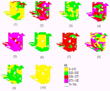
Figure 1. Habitat Suitability Index maps (1) barred owl (2) bobcat (3) brown thrasher (4) downy woodprcker (5) eastern cottontail (6) fox squirrel (7) gray squirrel (8) hairry woodpecker (9) northern bobwhite (10) pileated woodpecker (11) eastern wild turkey
Contrary to grat squirrel, fox squirrel was low in HSI. All of the cells had a HSI value for less than 0.5 (Figure 1). This was mainly due to the distance to available grain in this large forested area. Barred owl had low HSI value for most of the cells (Fig 1), more than 74 percent of the area. This result was a function of habitat variables which measured the number of big trees. Brown thrasher also had low HSI values (Fig 1). The high HSI value cells occurred where the canopy coverage was lower. Eastern wild turkey was low on HSI values (Figure 1). About 95 percent of the cells had HSI value lower than 0.5 (Table 2). This was mainly because of the optimum herbaceous coverage for eastern wild turkey was not provided by Compartment One. Northern bobwhite required low, dense woody vegetation and grassy areas. Therefore, the HSI value of northern bobwhite was low in Compartment One. Pileated woodpecker had the lowest HSI value among the 11 selected species. It required mature, dense forest with large snags, which was not available in Compartment One (Figure 1). The HSI value for the hairy woodpecker ranged from 0 to 1 (Figure 1). However, there was a big gap between the low value and high value cells. This was because of the number of very large snags per hectare required in the HSI model, a stand with a few large snags could have very high SI value while a stand with no large snags had a SI value of 0. For each species, the factor that dominates the final HSI value differs. However, the species that are low in HSI and high in HSI have some common characteristics. For species that prefer open forests such as fox squirrel and turkey, the HSI value is low because Compartment One is a dense forest. Early successional species such as northern bobwhite and brown thrasher that require low dense woody vegetation with a less dense overstory canopy have low HSI values. The optimum habitat of later successional species such as pileated woodpecker, barred owl, and turkey requires more large trees then is currently provided by Compartment One. Species with high HSI values tend to prefer mid-successional habitat. The optimum habitat of species such as downy woodpecker, eastern cottontail and gray squirrel require dense forest with nearly closed canopies, abundant understory cover with moderate shrub and herbaceous coverage (20-50%), and existence of some small snags. However, there are species with very specific needs. The hairy woodpecker, for example, prefers fairly large snags and large trees and its HSI values vary widely over Compartment One (Figure1).
| Species | Poor Habitat | Good Habitat | ||
| (Hectare) | (%) | (Hectare) | (%) | |
| Barred owl | 25,807 | 74.22 | 8,962 | 25.78 |
| Bobcat | 8,604 | 24.75 | 26,165 | 75.25 |
| Brown thrasher | 34,573 | 99.44 | 196 | 0.56 |
| Down woodpecker | 9,311 | 26.78 | 25,458 | 73.22 |
| Eastern cottontail | 0 | 0 | 34,769 | 100 |
| Fox squirrel | 34,769 | 100 | 0 | 0 |
| Gray squirrel | 5,528 | 15.90 | 29,241 | 84.10 |
| Hairy woodpecker | 19,015 | 54.69 | 15,754 | 45.31 |
| Northern bobwhite | 34,769 | 100 | 0 | 0 |
| Pileated woodpecker | 34,769 | 100 | 0 | 0 |
| Turkey | 32,937 | 94.73 | 1,832 | 5.27 |
5. Conclusions
A quantitative basis for management decisions may reduce the perception of subjective bias in decision making. This study provides a possible quantitative way to monitor management practices for ecosystem management by using HSI models. HSI models quantify habitat quality and permit consideration of wildlife along with other aspects of project planning, such as engineering and economics. They allow assessments of resultant changes in potential habitat quality and availability for selected wildlife species. This study's major contribution is the HIS incooperating spatial reseasoning and the redevelopment of spatially computed HSI. The use of a moving window that represents an animal's home range enabled the spatial evaluation of the habitat condition home range by home range. Thus, the HSI value of the each cell reflects the habitat condition of each species' home range, not the condition of one pixel. The moving window approach assessed the conditions of the home range at each point within each stand. Therefore, the automated HSI is not an assessment of the forest condition at each point but an assessment of habitat conditions of the home range (moving window). Futhermore, HSI habitat map shows the spatial distribution of poor habitat areas that need management attention and the good habitat areas that the manager may want to be careful about when harvesting or other activities are implemented.
6. Bibliography
- Allen, A.W. 1982. Habitat Suitability Index Models: Fox Squirrel.
U.S. Dept. Int., Fish Wildl. Serv. FWS/OBS-82/10.18. 11pp.
- Allen, A.W. 1982. Habitat Suitability Index Models: Gray Squirrel.
U.S. Dept. Int., Fish Wildl. Serv. FWS/OBS-82/10.19. 11pp.
- Allen, A.W. 1984. Habitat Suitability Index Models: Eastern
Cottontail. U.S. Dept. Int., Fish Wildl. Serv. FWS/OBS-82/10.66. 23pp.
- Allen, A.W. 1987. Habitat Suitability Index Models: Barred Owl. U.S.
Dept. Int., Fish Wildl. Serv. FWS/OBS-82/10.143. 17pp.
- Boyle, K.A., and T.T. Fendley. 1987. Habitat Suitability Index
Models: Bobcat. U.S. Fist Wildl. Serv. Biol. Rep. 82(10.147). 16pp.
- Cade, B.S. 1986. Habitat Suitability Index Models: Brown Thrasher.
U.S. Dept. Int., Fish Wildl. Serv. FWS/OBS-82/10.118. 14pp.
- Carroll, C. Ronald and Gary K. Meffe. 1994. Management to Meet
Conservation Goals: Applications in Gary K. Meffe and C. Ronald Carroll,
book, Principles of Conservation Biology.
- Eaton, Stephen W. 1992. Wild Turkey. The birds of North America, No.
22. 21pp.
- Grumbine, R. Edward. 1994. What is Ecosystem Management?
Conservation Biology 8(1):27-38.
- Irland Lloyd C. 1994. Getting from Here to There: Implementing
Ecosystem Management on the Ground. J. of Forestry 92(8):12-17.
- Noss, Reed F. and Allen Y. Cooperrider. 1994. Saving Nature's
Legacy: Protecting and Restoring Biiodiversity. Island Press,
Washington, D.C.
- Schroeder, R.L. 1982. Habitat Suitability Index Models: Downy
Woodpecker. U.S. Dept. Int., Fish Wildl. Serv. FWS/OBS-82/10.38. 10pp.
- Schroeder, R.L. 1982. Habitat Suitability Index Models: Pileated
Woodpecker. U.S. Dept. Int., Fish Wildl. Serv. FWS/OBS-82/10.39. 15pp.
- Schroeder, R.L. 1985. Habitat Suitability Index Models: Eastern Wild
Turkey. U.S. Dept. Int., Fish Wildl. Serv. FWS/OBS-82/10.106. 33pp.
- Schroeder, R.L. 1985. Habitat Suitability Index Models: Northern
Bobwhite. U.S. Dept. Int., Fish Wildl. Serv. FWS/OBS-82/10.104. 32pp.
- Schwartz, Charles W., and Elizabeth R. Schwartz, 1981. The Wild
Mammals of Missouri. University of Missouri Press and Missouri
Department of Conservation, 356pp.
- Sousa, Patrick J. 1987. Habitat Suitability Index Models: Hairy
Woodpecker. U.S. Dept. Int., Fish Wildl. Serv. FWS/OBS-82/10.146. 19pp.
- USDA. 1994. An Ecological Basis for Ecosystem Management. USDA
Forest Service, General Technical Report RM-246. Washington DC. 22pp.
- Whittaker, R. H. 1956. Vegetation of the Great Smoky Mountains. Ecol. Monogr. 26:1-80.