| GISdevelopment.net ---> AARS ---> ACRS 2000 ---> Environment |
Applying AVHRR Data to
Estimate and Monitor Aerosol Optical Thickness
Tang-Huang Lin* and
Gin-Rong Liu**
* Graduate Student, Institute of Space Science
National Central University.
** Professor, Center for Space and Remote Sensing Research
National Central University
Chung-Li, Taiwan 320
E-mail:grliu@csrsr.ncu.edu.tw
* Graduate Student, Institute of Space Science
National Central University.
** Professor, Center for Space and Remote Sensing Research
National Central University
Chung-Li, Taiwan 320
E-mail:grliu@csrsr.ncu.edu.tw
Key Words: Remotely sensed data, Atmospheric effect, Contrast reduction method
Abstract
Owing to the existence of atmosphere, the remotely sensed data observed from satellite are affected by the atmospheric effect. The actual information of earth surface are showed only while the effects are correctly removed. Basically the effects are dependent on the atmosphere conditions. In the visible and near IR spectral, the effects are mainly caused by the scattering of atmosphere molecular and aerosol. That is, the aerosol parameters can be retrieved from the remotely sensed data. So, this study improved the aerosol optical depth method developed by previous studies, to retrieve the aerosol optical depth by using AVHRR data. The results revealed that the improvements proposed by this study was accuracy and practical. On the other hand, since the aerosol concentration in the atmosphere is one significant index of the air quality, the distribution of air pollution seems can be monitored effectively with remote sensing data. Therefore, the application of the retrieved aerosol characters for environmental monitoring, such as air pollution, smoke, or dust detection, is also an important sub-topic in this research.
1. Introduction
In the visible and infrared spectral region, the atmospheric effects mostly come from the atmospheric molecular and aerosol scattering. Generally, these effects are not easy to corrected accurately although we know that they blur the ground truth information, especially for the part of aerosol scattering. There are two main methods have been used for atmospheric effects correction with remote sensing data. One is to pick up low and stable reflective objects, such as clear water body or dark dense vegetation (DDV) targets as the path radiance estimation reference, to reduce the aerosol optical parameter estimation error due to the uncertainty of object reflectance(Ahern et al., 1977; Liu et al., 1996). The other is so-call the "contrast-reduction" method. Assuming that the surface target reflectance are not changed, the aerosol optical parameter could be estimated by the radiance difference of satellite observations in a series times with a reference datum. Based on that, Tanre et al. constructed the Structure Function (SF) method with the Landsat TM images and got satisfying results in 1988. Holben et al. (1992) also got good results using AVHRR data for aerosol optical depth retrieval by SF method. Sifakis et al. (1992 and 1998) applied the contrast method for SPOT and Landsat TM satellite image to estimate the aerosol optical parameter and monitor the air pollution over urban area.
In this study, the SF method is applied to estimate the aerosol optical depth over Taiwan area from AVHRR data, but some anomalies of the structure function distribution pattern were appeared. The anomalies probably due to the sensor observing geometry, the change of landcover in the multi-temporal images and terrain effect and would induce the significant errors in aerosol optical depth estimation. In order to avoid such errors, the study would introduce the "optimal position number" to remove the distribution anomalies(Liu et al., 1997). The maximum error of estimated aerosol optical parameter is reduced from 61% to 24% after the "optimal position number" is adopted in this study. The result also shows that this improvement is one of the crucial steps in estimating aerosol optical parameter. Not only the estimation accuracy is improved significantly when the "optimal position number" is employed, but also make the structure function more practical.
2. Methodology
Assume the ground surface observed by satellite is Lambertian, the equivalent ground reflectance observed by satellite is?*, and can be expressed as (Tanre et al., 1988)
where?* is equivalent ground reflectance, , is solar zenith angle, and is sensor zenith angle, is atmospheric reflectance, is relative azimuth angle between solar and sensor, is atmospheric optical depth, ground surface reflectance, T is total transmittance from solar to ground surface, s is atmosphere albedo, is mean surface reflectance, is diffuse transmittance from surface to sensor. Under the following conditions: (1) Ignore the multi-reflectance activities between earth surface and atmosphere; (2) The surface is unchanged in time; (3) The mean surface reflectance is constant, then we can obtain:
where M is the structure function defined by Taner et al.(1988),

and Function[ta ] = T(µs)exp[-2t/µv]
The parameters of t1 and t2 indicate the two different observation time. From Equation (2), it is clear that the aerosol optical depth will get different values in different distance, d, unless the ration of structure function is constant. Basically the mean ration of d=1 to d=10 is used in the general cases. In some cases, the errors of estimated aerosol optical depth are large when the correlation of ration in the different d number is low.
Applied Equation (3) defined by Tanre et al. to estimate the optical depth over the northern Taiwan area with AVHRR visible data, the structure function distribution of neighboring pixels with different d numbers is showed in Figure 1. Assume the difference of surface reflectance is increasing when the distance is increasing, the structure function will is increasing when d number is increasing and has the similar distribution pattern (Tanre et al., 1988; Holben et al., 1992). But the structure functions of different dates were changed significantly in Figure 1. It may be caused by the terrain effect, the complex canopy in Taiwan area and the satellite geometric observation. This anomaly will influence the retrieved aerosol optical depth strongly. This study used the result of statistical analysis for determining the "optimal position number" to discard the anomalous structure functions.
Figure 2(a) and 2(b) are the histogram of AVHRR channel 1 digital count difference for different d values on 6 and 19 November. Generally the reflectance differences distribution of the neighboring pixels are similar to normal distribution. In Figure 2(a), the distribution is quite irregular when d=5, while the distribution is regular and similar to the right wing of normal distribution in Figure 2(b). This anomaly would influent the structure function pattern as illustrated in the Figure 1, square symbols bending anomaly after d=5 on 6 November. Then the "optimal position number" is set at d=5 in this case study to reduce the errors induced by the structure function anomalies.
3. Results
This study used one set of multi-temporal NOAA-14 AVHRR data to estimate the atmospheric aerosol optical depth. The data set includes 6 AVHRR images acquired during November, 1997 over Chung-Li, Taiwan, shown in Table 1. The size of tested area in this study was about 25 x 25 km at the Northern Taiwan, and landuse includes urban, rural, agricultural and tree area. This tested area is over the neighboring area of National Central University (NCU), and the sunphotometer observation site(at NCU). The ground measured aerosol optical depth were used for reference and as the checked data to confirm our estimated results.
The results of aerosol optical depth estimated by not using and using "optimal position number" are listed in Table 2 and 3, respectively. The comparison with the sunphotometer measurements showed that the errors induced by the anomalies of structure function distribution were obvious reduced and the maximum errors were reduced from 61% to 24%. It revealed that the application of the "optimal position number" really could improve the estimation accuracy significantly.
4. Conclusion
The induce of the "optimal position number", which can reduce errors efficiently, is one of important procedures of applying structure function method to retrieve aerosol optical depth. The result in this study reveals that this improvement is very useful in promising the estimation accuracy and extends the application of the relative satellite images in the different area. Meanwhile, it can reduce the sensitivity of data acquiring time, especially for more longer time interval data, and prolong the applied time interval of referred observation data. Of course, the limitation of the "optimal position number" should be investigated further. This improvement also can be applied in some high time-resolution geostationary satellite images, such as GMS and GOES, to estimate the relative air quality parameters for air quality monitoring.
References
- Ahern F. J., D. G. Goodenough, S. C. Jain, V. R. Rao, and G. Rochon, 1977: Landsat atmospheric corrections at CCRS, In Proceedings of the Fourth Canadian Symposium on Remote Sensing, Quebec City, May, 583-595.
- Holben, E. Vermot, Y. J. Kaufman, D. Tanre, and V.Kalb, 1992: Aerosol Retrieval over Land from AVHRR Data-Application for Atmospheric Correction. IEEE Trans. on Geoscience and Remote Sensing, Vol. 30, No. 2, pp. 212-222.
- Liu C. H, A. J. Chen, and G. R. Liu, 1996: An Image-based Retrieval Algorithm of aerosol Characteristics and Surface Reflectance for Satellite Images. INT. J. Remote Sensing, Vol. 17, No. 17, 3477-3500.
- Liu G. R, T. H. Lin, and A. J. Chen, 1997: An Improved Method to Determine Aerosol Optical Depth from SPOT Data. COAA '97-First International Ocean-Atmosphere Conference, 18-19 Oct 1997, Washington, D. C., USA.
- Sifakis N. I. and P. - Y. Deschamps , 1992: Mapping of Air Pollution Using Satellite Data. Photogrammetric Engineering & Remote Sensing, Vol. 58, No. 10, 1433-1437.
- Sifakis N. I., N. A. Soulakellis, and D. K. Paronis, 1998: Quantitative mapping of air pollution density using Earth observations: a new processing method and application to an urban area. INT. J. Remote Sensing, Vol. 19, No. 17, 3289-3300.
- Tanre D., P. Y. Deschamps, C. Devaux, and M. Herman, 1988: Estimation of Saharan Aerosol Optical Depth from Blurring Effects in Thematic Mapper Data. J. Geophys Res., Vol. 93, No. D12, pp 15955-15964.
Table 1. The observation geometry of NOAA-14 AVHRR satellite of the five observations using in this study. (* : reference date)
| Orbit number | Date | Local Time |
Satellite Zenith Azimuth |
Solar Zenith Azimuth | ||
| 14700 | 1997/11/06* | 06:40 | 58 | 193 | 58 | 228 |
| 14714 | 1997/11/07 | 06:29 | 48 | 186 | 56 | 224 |
| 14756 | 1997/11/10 | 05:56 | 3 | 165 | 52 | 215 |
| 14770 | 1997/11/11 | 05:45 | 23 | 158 | 51 | 212 |
| 14883 | 1997/11/19 | 05:58 | 1 | 166 | 54 | 215 |
| 14897 | 1997/11/20 | 05:47 | 21 | 159 | 53 | 213 |
Table 2. The comparison of the aerosol optical
depth estimated by sunphotometer data and AVHRR Channel 1 data, while the
"optimal position number" was not used. (* : reference date)
| Date |
AVHRR CH1 (580-680 nm) |
Sunphotometer measurement |
Error/Percentage
|
| 1997/11/06* | 0.204 | 0.204 | ---- |
| 1997/11/07 | 0.473 | 0.346 | 0.127 / 38% |
| 1997/11/10 | 0.345 | 0.214 | 0.131 / 61% |
| 1997/11/11 | 0.430 | 0.275 | 0.155 / 56% |
| 1997/11/19 | 0.489 | 0.483 | 0.006 / 1% |
| 1997/11/20 | 0.349 | 0.240 | 0.109 / 45% |
Table 3. Same as Table 2, except the "optimal position
number" was used.
| Date | AVHRR CH1(580-680 nm) | Sunphotometer measurement | Error/Percentage |
| 1997/11/06* | 0.204 | 0.204 | ---- |
| 1997/11/07 | 0.431 | 0.346 | 0.085 / 24% |
| 1997/11/10 | 0.242 | 0.214 | 0.028 / 13% |
| 1997/11/11 | 0.347 | 0.275 | 0.028 / 10% |
| 1997/11/19 | 0.474 | 0.483 | 0.009 / 2% |
| 1997/11/20 | 0.254 | 0.240 | 0.014 / 6% |
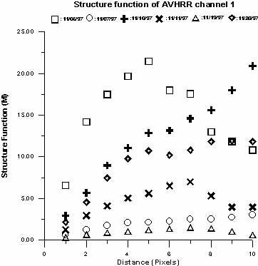
Figure 1. The structure functions derived from AVHRR-14 Channel 1 data, acquired on 6 dates, with different distances, d.
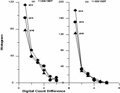
Figure 2. The comparison of digital count different histogram of AVHRR Channel 1 data acquired on 1997/11/06 and 1997/11/20 with d=4, 5 and 6. Figure 2(a) shows the curve of d=5 shifting right hand side obviously. It means that the difference of ground reflectance property in this AVHRR data is large. The difference is not found in Figure 2(b).