| GISdevelopment.net ---> AARS ---> ACRS 2000 ---> Digital Photogrammetry |
Multi-Resolution approach to
Radargrammetric Digital Elevation Models Generation
Xiaojing HUANG, Leong Keong
KWOH and Hock LIM
Centre for Remote Imaging, Sensing and Processing
National University of Singapore
SOC1 Level 2, Lower Kent Ridge Road, Singapore 119260
Fax: (65)7757717
Email:crshxj@nus.edu.sg
Key WordsCentre for Remote Imaging, Sensing and Processing
National University of Singapore
SOC1 Level 2, Lower Kent Ridge Road, Singapore 119260
Fax: (65)7757717
Email:crshxj@nus.edu.sg
Digital Elevation Models, Radargrammetry, Correlation
Abstract
In this paper, we present our work in Digital Elevation Models (DEM) generation with RADARSAT stereopairs, usually form from S2 and S6 standard beam modes, using radargrammetric technique. We introduced a weighted block window for the matching of corresponding patches and a hierarchical multi-resolution approach to improve the DEM generation robustness. Prior to DEM generation, an imaging model based on the satellite and target geometry, and signal acquisition time for RADARSAT has been developed, and the model parameters have been refined to match the local terrain with ground control points (GCPs).
1. Introduction
DEM of a region can be generated from stereopairs of satellite images. In tropical areas where cloud free optical images are hard to acquire, DEM generation with radargrammetry using high resolution spaceborne synthetic aperture radar (SAR) images, such as RADARSAT images, is a potential alternative. In this paper, we described the system we developed at CRISP for DEM generation from RADARSAT stereopairs. The main processing steps involved are (a) establishing the SAR imaging model and determining the parameters of the imaging models, (b) automatic DEM generation applying a weighted block window digital correlation and implementing a hierarchical multi-resolution approach.
SAR Imaging Model
In a SAR image, the location on the ground of an image sample (u, v) can be derived from knowledge of the sensor position and velocity [1]. The pixel coordinate u is related to the slant range r from the sensor to the corresponding point on the ground. While the line coordinate v is related to the azimuth time s at which the pulse of the corresponding line is transmitted. These relationships can be expressed as follows:
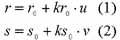
where r0 is the slant range of the first pixel in the image, k0 is the scaling factor in the range direction, s0 is the azimuth time of the first line in the image, and ks0 is the scaling factor in the azimuth direction. The preliminary values of r0 , kr0 , s0 and ks0 can be obtained from the RADARSAT product leader file.
The SAR range r and line time s of any target is further related to the sensor as follows:
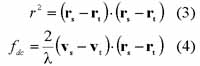
where rs, vs are sensor position and velocity vectors, and rt, vt are target position and velocity vectors. fdc is the Doppler centroid frequency, and l is the radar wavelength. For RADARSAT SGF images, fdc is zero since the image is resampled to the zero-Doppler. The target velocity can be determined from the target position since the target is on the earth surface. The sensor position and velocity can be derived from azimuth time s and satellite state vectors given in the image leader file.
Equations (1) - (4) describe the imaging model we use for a SAR image. All imaging parameters can be obtained from the image product leader file. To optimize the imaging model for the local area of interest, some parameters can be refined with GCPs. We choose to only refine equation (1) and (2) with the following expressions:
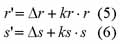
where Dr and kr are the shift and scaling factor of image slant range, respectively, D s and ks are the shift and scaling factor of image azimuth time, respectively, r' and s' are the corrected slant range and azimuth time, respectively. There are thus a total of 4 parameters to be refined for each image. These 4 parameters are solved by least square adjustment techniques, using at least 2 GCPs.
To verify the correctness of the imaging model, we use them to terrain geocode a RADARSAT S2 image (fig 1) and a RADARSAT S7 image (fig 3) of Lantau Island (Hong Kong) with available DEM. The parameters of the imaging model for each image were refined using GCPs obtained from topographic maps. The good agreement of the terrain corrected geocoded images shown in figure 4 ( the S2 geocoded image shown in red and the S7 geocoded image shown in cyan) shows the correctness of the model.
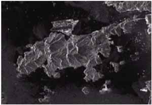
Figure 1. Lantau Island in RADARSAT SGF image of S2 mode acquired on 25 Dec 1996
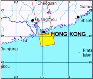
Figure 2. (below) Lantau Island location map.
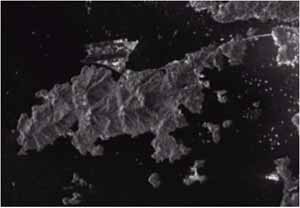
Figure 3. Lantau Island in RADARSAT SGF image of S7 mode acquired on 28 Dec 1996.
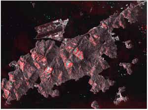
Figure 4. Two images match very well after geocode to accurate topographic map (red for S7 mode, green and blue for S2 mode).
The underlying principle for generating the DEM is to find, for each X,Y coordinates, a height H where the normalized cross correlation of two image patches, one from each images, is highest within a range of heights. The location of each image patch is computed from the refined imaging model. A problem in correlating SAR imagery is that there are usually some very dominating high intensity features amongst the majority of average intensity features. When we choose any patch, the correlation results will be biased to these strong intensity features, even though they may be at the far edges or corners of the patch. We reduce this problem by introducing a weighted block window to minimize the contribution of the edge pixels in the correlation computation. The weighted block window chosen is the Welch window [4] in two dimensions. The weighted window wi in one dimension of pixel i can be expressed as follows:
wi = 1 - [ ( i - N - 1) / ( N + 1 )]2
(7)
where N is the half window size in one dimension. The full window size in one dimension is 2N+1. Figure 5 shows the weighted window in one dimension with N = 19. The weighted window wij in two dimension ( i, j ) is:
wij = wi × wi
(8)
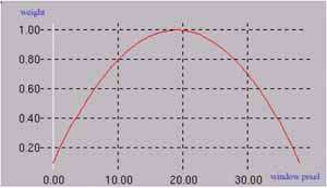
Figure 5. The weighted window in one dimension with N = 19.
Hierarchical Multi-Resolution Approach
To improve the robustness of the DEM generation processing, a hierarchical multi-resolution approach (fig.6) is implemented. The original stereo pair of imagery (12.5m/pixel) were averaged over 16´16 (200m/pixel), 4´4 (50m/pixel) and 2´2 (25m/pixel) pixel-windows. A preliminary DEM is first computed from the correlation of the lowest resolution (200m/pixel) image pair. For the higher resolution computation, the DEM computed at the previous step is used to carry out a geometric correction of the image pair to enhance correlation, hence more accurate height determination. The advantage of using this hierarchical multi-resolution matching technique is that it is easier to find the correct matching of the reduced resolution images because of the removal of the speckle noise and detailed features in the block window.
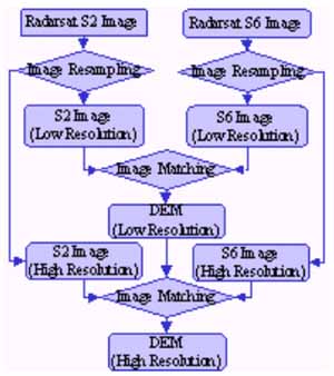
Figure 6. Hierarchical multi-resolution DEM approach
Test Site and DEM Generation
The hierarchical multi-resolution DEM approach was tested with two descending RADARSAT images of S2 and S6 beam modes (fig. 7 and 8) over Brunei. The detailed image description is listed in table 1. The pair of imagery (12.5m/pixel) were averaged over 16´16 (200m/pixel), 4´4 (50m/pixel) and 2´2 (25m/pixel) pixel-windows. The lowest resolution (200 m/pixel) DEM (fig. 9) of the area was first generated from the 200m/pixel image layers. The 50m/pixel resolution DEM (fig. 10) of the same area was later generated from 50m/pixel image layers by using the terrain information of previous DEM. Finally, the highest resolution DEM (fig. 11) of 20m/pixel of the same area was generated from 25m/pixel image layers by using more detailed terrain information of previous DEM layer. An attempt to generate 10m/pixel resolution DEM by using the original imagery did not produced satisfactory results, probably because of the heavily scattered speckle noise at that resolution that causes de-correlation of the image patches.
Table 1. The description of Radarsat stereo imagery used in the DEM generation
| Stereo Pair | Image Format | Beam Mode | Incidence Angle (degree) | Orbit | Date | Image Pixel (12.5m/pixel) |
| Image No. 1 | SGF | S2 | 23.8 – 31.1 | 12110 | 28 Feb 1998 | 8953×9000 |
| Image No. 2 | SGF | S6 | 41.4 – 46.7 | 11381 | 8 Jan 1998 | 8675×9000 |
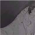 Figure 7. (above) Radarsat image (S2 mode) acquired on 28 Feb 1998. © CSA 1998 |
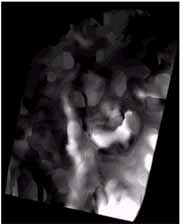 Figure 9. DEM with 200m/pixel resolution in an area of 80×100 km2.Map projection: UTM 50N Datum: GRS 1980 |
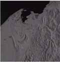 Figure 8. (above) Radarsat image (S6 mode) acquired on 8 Jan 1998.© CSA 1998 | |
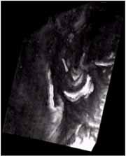 Figure 10. DEM with 50m/pixel resolution in the same area.Map projection: UTM 50N Datum: GRS 1980 |
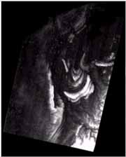 Figure 11. DEM with 20m/pixel resolution in the same area.Map projection: UTM 50N Datum: GRS 1980 |
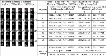
An example of the correlation at a range of height in the generation of 25m/pixel resolution DEM is shown on figure 12. The locations of the block window centres in the image layers are listed on table 2. It can be seen that a 5m change in height causes a relative shift of 0.22 pixel in the image pair, i.e. 5.5m in distance. As the resolution of the RADARSAT standard image used is 25m, it may suggest that the accuracy of the generated DEM, if the matching accuracy is 1 pixel, will be about 23m.
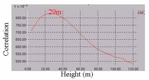
Figure 12. Correlation of weighted block windows changes with a range of height
Table 2. Image blocks and center pixel coordinates for matching.
Conclusion
The imaging model based on physical imaging parameters of the SAR is described. The parameters of our model can be refined with 2 GCPs or more. A weighted block window has been implemented to improve the digital correlation of the matching patches and a hierarchical multi-resolution approach is implemented to increase the robustness of the DEM generation process. The high disparity between the DEM generated from RADARSAT and that from SPOT has a standard deviation of 26 meters. More work will be done to reduce this disparity.
References
- Curlander, John C. and Mcdonough, Robert N., "Synthetic Aperture Radar, Systems & Signal Processing", p370-377, 1991.
- J.S. Greenfeld, "An operator-based matching system", Photogrammetric Eng. Remote Sensing, 57(8), 1049-1055, August 1991.
- Thierry TOUTIN, "SAR image sampling on DEM generation", IEEE 2000 International Geoscience and Remote Sensing Symposium, volume III, 794-796, July 2000.
- Willian H. Press, etc., "Numerical Recipes in C", p554.
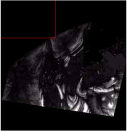
Figure 13. DEM generated from SPOT stereopair with IMAGINE Orthomax software.
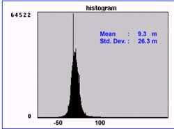
Figure 14. The height disparity map between the DEMs generated from RADARSAT stereo pair and SPOT stereo pair.
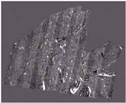
Figure 15. Histogram of the disparity map.