| GISdevelopment.net ---> AARS ---> ACRS 1999 ---> Water Resources |
Flood Predicition from
LANDSAT Thematic Mapper Data and Hydrological Modeling
Mohd. Ibrahim Seeni Mohd.
& Mohamad Adli bin Mansor
Dept. of Remote Sensing
Faculty of Geoinformation Science & Engineering
Universiti Teknologi Malaysia
81310 Skudai, Johor Bahru, Malaysia.
Tel: 607-5502880, Fax: 607-5566163
E-mail: mism@fksg.utm.my
AbstractDept. of Remote Sensing
Faculty of Geoinformation Science & Engineering
Universiti Teknologi Malaysia
81310 Skudai, Johor Bahru, Malaysia.
Tel: 607-5502880, Fax: 607-5566163
E-mail: mism@fksg.utm.my
Remote sensing techniques have been used in various applications including agriculture, forestry, oceanography and environmental studies. This paper reports on a study that has been carried out using remote sensing techniques and hydrological modelling for flood prediction in the Klang Valley. The remote sensing satellite data that have been used is the Landsat-5 Thematic Mapper (TM) data whilst the flood prediction is based on the U.S. Soil Conservation Service Technical Release 55 (SCS TR-55) model. This model involves the calculation of runoff from Curve Numbers (CN) that relate to land use, soil type, hydrological condition and soil moisture. In the determination of runoff, land use information are derived from the Landsat-5 TM data and land use maps. The runoff values were used in the calculation of concentration time, peak discharge and bankfull discharge. The peak discharge was calculated by the graphical method of SCS TR-55 model whilst the bankfull discharge was derived from the slope area method. Flood occurrence was determined by comparing the peak discharge values with bankfull discharge values. Flooding occurs if the peak discharge exceeds the bankfull discharge. In the study, watershed areas were generated and the area that would be flooded for specific amount of rainfall were determined using remote sensing techniques and the SCS TR-55 model. The results that were obtained are encouraging and indicate the potential of using remote sensing techniques with hydrological modelling for flood prediction. (Keywords : Remote sensing, hydrological modelling, floods)
Introduction
Flood is a major problem especially for people who live in low lying areas. Floods can cause death and at the same time bring damage to properties such as houses, buildings, plantation, livestock, etc. Studies of floods using remote sensing techniques usually involve delineating flooding areas. For example, Philipson et al. (1980) used Landsat Thematic Mapper (TM) data to map the flood boundary for Black River in the U.S.A. This study used visual interpretation techniques of band 7 (0.8 - 1.1 µ m) Landsat TM data. Other studies in flood delineation can be found in Sollers et al. (1978) and Kalensky et al. (1979). Remote sensing techniques are also used to monitor lake and swamp areas. Barret et al. (1982) used remote sensing techniques to monitor large lake and swamp such as Lake Chat and Okowango swamp in South Africa. In this study they used the visible and infrared bands of the Meteosat data.
Generally, flood is an important subject of study in hydrology and hydrologists are able to predict floods by using hydrological modelling. The data that are needed in flood prediction are rainfall, land use, topography information etc. These data are generally derived from field observations which are costly and time consuming. The use of remote sensing techniques can decrease the cost of data acquisition. Remote sensing can also provide up-to-date data or information for large areas in a short time compared to traditional methods (Philipson et al. 1980, U.S. Department of Agriculture, 1986). The U.S. Department of Agriculture uses remote sensing techniques in determining watershed geometry, drainage network, soil moisture data and land use information. Various studies have also been done in determining runoff coefficient using remote sensing data (Bondelid et al. 1981, Engman and Sing 1981 and Hill et al. 1987). Engman and Sing (1981) reported that remote sensing is rapidly becoming an important source of data and information for hydrological modelling. Ochi et al.(1989), have used remote sensing data in flood damage forecasting based on flood flow modelling. Normalized vegetation index (NVI) from remote sensing data and slope gradient were used to calculate runoff ratio. The flood flow modelling was later used in simulation study for flood movements in various types of vegetation.
This paper reports on the use of the Landsat-5 Thematic Mapper (TM) data and the U.S. Soil Conservation Service Technical Release 55 (SCS TR-55) hydrological model in the prediction of floods in the Klang Valley and its surrounding areas.
Study Area
The Klang Valley and its surrounding areas have been selected for the study. The area falls within the coordinates 366 000mE, 360 000mN and 444 000mE, 330 000mN (refer figure 1). This area is chosen since it is in a valley surrounded by hills with some major rivers flowing through the area. Many locations in the area are also prone to flooding during heavy rainfall.
FIGURE 1. Study area of Klang Valley and its surrounding areas.
Remote Sensing Data and Other Ancillary Data
The remote sensing data that was used is the Landsat-5 TM satellite data (see figure 2). The satellite data is relatively cloud free and excellent for deriving various information required in the study. Other data that were collected are rainfall data, soil type data and information on hydrological condition.
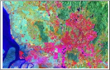
FIGURE 2. Landsat-5 TM image of study area.
Satellite Data Processing
Remote sensing data usually contain both systematic and nonsystematic geometric errors. These errors may be divided into two classes: those that can be corrected using data from platform ephemeris and knowledge of internal sensor distortion, and those that cannot be corrected with acceptable accuracy without a sufficient number of ground control points (Jensen, 1986)
Geometric Correction
Geometric correction is undertaken to avoid geometric error from a distorted image. In this study, the Landsat-5 TM image was rectified using ground control point (GCP). The GCPs were taken from topographical map of the study area. Cubic convolution resampling technique was used in the geometric correction which results in sharpening as well as smoothing the image. Thirteen GCPs were used in the geometric correction which produced root-mean-square error of about 10 meters in Easting and Northing.
Image Classification
Image classification was carried out to classify the land use type in the study area. This information is required so that specific Curve Number (CN) can be assigned to the specific land use in the hydrological modelling described in section 5.0. The supervised classification technique using the maximum likelihood classifier was used. In a supervised classification, the identity and location of some of the land cover type, such as urban, agriculture, wetland and forest are known a priori through a combination of field work, analysis of aerial photography, maps and personal experience (Jensen 1986). In this study, the training areas for supervised classification were identified from topographic maps and existing land use maps. Ten classes of land cover have been identified in this study area, namely, (1) mangrove, (2) urban or built up areas, (3) oil palm plantation, (4) coconut plantation, (5) forest, (6) open areas, (7) rubber plantation, (8) paddy, (9) water body and (10) grassland. The overall classification accuracy is about 86%.
Hydrological Modelling
In this study the U.S Soil Conservation Service Technical Release 55 (SCS TR-55) hydrologic model has been used to predict floods in the Klang Valley and its surrounding areas. This model presents a simplified procedure for estimating runoff and peak discharge in small watersheds (U.S. Department of Agriculture, 1986). There are several calculations involved that include the determination of runoff by SCS TR-55 Curve Number (CN) method, concentration time, peak discharge, and bankfull discharge.
The Determination of Runoff
The U.S. SCS TR-55 method uses the Curve Number method to estimate runoff from storm rainfall. This method starts with the determination of CN, which depends on the watershed's soil and cover conditions. The watershed's soil and cover conditions in SCS TR-55 model represent the hydrologic soil group, cover type, treatment and hydrologic condition.
The SCS TR-55 runoff equation used is : -
where, Q = runoff (in)
P = rainfall (in)
s = potential maximum retention after runoff begins (in)
Ia = Initial abstraction (in).
Initial abstraction is all losses before runoff begins. Through studies of many small agricultural watersheds, Ia was found to be approximated by the following empirical equation (U.S. Department of Agriculture, 1986) : -
Ia= 0.2s…………………(2)
By substituting the equation (2.) into equation (1.), gives : -
s is related to the soil and cover conditions of watershed through CN and s related to CN by : -
Based on the SCS TR-55 model, the Runoff Curve Number for the watershed's land cover, soil type and conditions in the study area is given in Table 3.
TABLE 3. CN for each land cover in study area
| Land Cover / Land Use | Curve Number (CN), for Hydrological Soil Group - B |
| Water Body | 100 |
| Open Area | 79 |
| Mangrove | 98 |
| Oil Palm | 60 |
| Coconut | 65 |
| Rubber | 66 |
| Forest | 55 |
| Urban or Built up area | 93 |
| Paddy | 79 |
| Grassland | 65 |
In this calculation a rainfall amount of 3.94 in was used based on 24-hour storm event for the study area. The runoff values (Q) estimated by SCS TR-55 CN method for each watershed in the study area is given in Table 4 whilst the watersheds are showed in Figure 4.
FIGURE 4. Watersheds in the study area.
TABLE 4. Runoff for each watershed
| Watershed | Runoff (Q) (in) |
| Wt1 | 0.8775 |
| Wt2 | 0.8369 |
| Wt3 | 0.8990 |
| Wt4 | 0.8478 |
| Wt5 | 0.9957 |
| Wt6 | 0.9811 |
| Wt7 | 1.7806 |
| Wt8 | 1.4120 |
| Wt9 | 2.2154 |
| Wt10 | 1.3406 |
| Wt11 | 2.5235 |
| Wt12 | 1.9504 |
| Wt13 | 2.2750 |
| Wt14 | 1.4303 |
| Wt15 | 1.8968 |
| Wt16 | 1.3493 |
| Wt17 | 1.2351 |
| Wt18 | 1.8337 |
| Wt19 | 1.8855 |
| Wt20 | 2.0648 |
| Wt21 | 1.6273 |
| Wt22 | 1.4428 |
| Wt23 | 1.1375 |
Determination of Concentration Time and Travel Time
Travel time (Tt) is the time of travel of water from one location to another in a watershed. Tt is a component of time of concentration Tc and Tc is the time for runoff to travel from the hydraulically most distant point of the watershed to a point of interest within the watershed. Tc is computed by summing all the Tt for consecutive components of the drainage conveyance system.
Tt is the ratio of flow length to flow velocity : -
where, Tt = travel time (hr)
L = flow length (ft)
V = average velocity (ft/s)
3600 = conversion from second to hours.
The average velocity (V), was computed by the Manning's equation :-
r = hydraulic radius (ft) and is equal to a/pw
a = cross sectional flow area (ft2 )
pw = wetted perimeter (ft).
S = slope of the hydraulic grade line (channel slope, ft/ft)
n = Manning's roughness coefficient for open channel flow.
The time of concentration (Tc) is the sum of Ttof the various consecutive flow segments,
Tc= Tt1+Tt2+……+ Ttm……………(7)
where, Tc = time of concentration (hr)
m = number of flow segment
Tt= travel time of a segment.
Table 5 shows the time of concentration for each watershed in the study area.
TABLE 5. The concentration time for each watershed
| Watershed | Area (mi2) | Flow Length (ft) | Concentration Time (hr) |
| Wt1 | 12.2709 | 31576.1455 | 3.4115 |
| Wt2 | 17.2671 | 43649.0935 | 5.2616 |
| Wt3 | 5.2742 | 19134.815 | 2.2029 |
| Wt4 | 6.5450 | 22340.1859 | 2.6725 |
| Wt5 | 35.8262 | 52883.9475 | 4.79074 |
| Wt6 | 9.5793 | 39302.9858 | 4.0881 |
| Wt7 | 1.3066 | 10667.9244 | 0.41365 |
| Wt8 | 7.6330 | 34744.5461 | 2.40227 |
| Wt9 | 1.3368 | 12939.6384 | 0.57828 |
| Wt10 | 19.5362 | 52520.3703 | 4.49168 |
| Wt11 | 1.7229 | 7979.3706 | 0.54646 |
| Wt12 | 7.6503 | 37255.777 | 1.59095 |
| Wt13 | 12.3727 | 35040.8425 | 3.5393 |
| Wt14 | 59.0031 | 62278.0685 | 6.76384 |
| Wt15 | 29.0425 | 59213.6906 | 5.16663 |
| Wt16 | 25.7438 | 90815.7426 | 6.47327 |
| Wt17 | 21.0961 | 90815.7426 | 3.79186 |
| Wt18 | 32.2196 | 58721.3330 | 6.95108 |
| Wt19 | 28.8111 | 36803.7179 | 3.85335 |
| Wt20 | 25.52 | 50864.0234 | 6.29147 |
| Wt21 | 38.0265 | 86440.2044 | 0.62849 |
| Wt22 | 117.4947 | 73481.3778 | 0.32320 |
| Wt23 | 2.6712 | 14059.0118 | 1.09378 |
Determination of Peak Discharge
The peak discharge was determined by SCS TR-55 graphical method. In this method, the peak discharge is calculated by : -
qp= qu Am QFp …………………(8)
where, qp = peak discharge (cfs)
qu= unit peak discharge
Am = drainage area (mi2)
Q = runoff (in)
Fp = pond and swamp adjustment factor.
The results of the peak discharge for each watershed are presented in Table 6.
Determination of Bankfull Discharge
The bankfull discharge was determined using the slope area method. In this method the equation that was used is : -
Qb=KÖ S ……………………(9)
where, Qb = bankfull discharge
K = average conveyance
ÖS = slope energy
K is defined by Manning's formula as: -
where, A = cross sectional flow area (ft2 )
R = hydraulic radius
n = Manning's roughness coefficient
Slope energy S can be calculated from equation as below: -
S = F/L ………………….……(11)
where, S = slope energy
F = changes in surface level
L = flow length
The results of bankfull discharge estimation are given in Table 6.
TABLE 6. Peak and bankfull discharge for each watershed in the study area
| Watershed | Peak Discharge | Bankfull Discharge |
| Wt1 | 1117.150 | 1109.554 |
| Wt2 | 1106.356 | 1244.394 |
| Wt3 | 647.216 | 1650.850 |
| Wt4 | 559.047 | 1711.801 |
| Wt5 | 3185.522 | 674.229 |
| Wt6 | 806.370 | 937.281 |
| Wt7 | 809.632 | 1039.900 |
| Wt8 | 1353.552 | 692.798 |
| Wt9 | 924.003 | 982.824 |
| Wt10 | 2294.264 | 642.578 |
| Wt11 | 1523.118 | 1482.749 |
| Wt12 | 2077.023 | 514.570 |
| Wt13 | 3968.853 | 942.209 |
| Wt14 | 5813.774 | 798.083 |
| Wt15 | 5437.167 | 617.865 |
| Wt16 | 2085.208 | 432.217 |
| Wt17 | 2567.798 | 1304.564 |
| Wt18 | 4070.095 | 1006.204 |
| Wt19 | 5720.246 | 970.127 |
| Wt20 | 3805.012 | 1278.227 |
| Wt21 | 6572.950 | 618.227 |
| Wt22 | 9154.677 | 862.108 |
| Wt23 | 643.258 | 1139.014 |
TABLE 7. Optimum rainfall for each watershed
| Watershed | Optimum rainfall (in) |
| Wt1 | 2.8 |
| Wt2 | 2.5 |
| Wt3 | 3.6 |
| Wt4 | 3.8 |
| Wt5 | 2.2 |
| Wt6 | 2.8 |
| Wt7 | 2.6 |
| Wt8 | 2.0 |
| Wt9 | 2.3 |
| Wt10 | 1.8 |
| Wt11 | 2.2 |
| Wt12 | 2.0 |
| Wt13 | 2.3 |
| Wt14 | 2.0 |
| Wt15 | 2.0 |
| Wt16 | 2.0 |
| Wt17 | 1.9 |
| Wt18 | 2.0 |
| Wt19 | 2.0 |
| Wt20 | 2.4 |
| Wt21 | 1.9 |
| Wt22 | 2.1 |
| Wt23 | 3.1 |
The watersheds that are susceptible to flooding were determined by comparing the peak and bankfull discharge for each watershed. Flooding occurs if the peak discharge exceeds the bankfull discharge. From Table 6, there are a number of peak discharges that exceed the bankfull discharges in several watersheds with the rainfall amount of 3.94 in. These watersheds will be flooded. The optimum rainfall amount for every watershed before flooding occurs can be determined from equation (1) and (8) by making P as an unknown. Table 7 shows the optimum rainfall for each watershed.
Discussions and Conclusion
The optimum amount of rainfall for each watershed has been presented in Table 7. The flood prone watershed can be determined from the optimum rainfall amount for each watershed. From Table 7, the watershed that is most prone to flooding is Wt10. This watershed is located in low lying areas with a major river Sg. Kelang flowing through it. The model that has been used is based on soil and land use for the United States. The use of this model for the Malaysian environment may not be very accurate since the value for some parameters may not be representative for the soil and land use in our environment.
From this study, it can be concluded that remote sensing techniques with suitable hydrological modelling can provide a useful technique for prediction of floods. Further studies with the use of digital elevation models can indicate the specific areas that are flooded within a watershed.
Acknowledgements
The authors wish to thank the Malaysian Meteorological Service for providing the rainfall data and the Department of Agriculture for providing information on land use and soil types.
References
- Barrett, E.C. and Curtis, L.F., (1982). Introduction To Environmental Remote Sensing (2nd Ed.), New York : Chapman and Hall.
- Bondelid, T.R., Jackson, T.J., McCuen, R.H., Sing, P.V. (Ed), (1981). “Estimating Runoff Curve Numbers Using Remote Sensing Data”. Applied Modeling in Catchment Hydrology. Water Resources Publication, U. S.A.
- Engman, T.E., Sing, P.V. (Ed), (1981). “Remote sensing Application in Watershed Modeling” ; Applied Modeling in Catchment Hydrology. Water Resources Publication, U.S.A. Hill, J. M., Singh, V. P. and Aminian, H., 1987. "A Computerized Data Base For Flood Prediction Modelling". Water Resources Bulletin. Vol. 23, No. 1.
- Jensen, J.R., 1986. Introductory Digital Image Processing : A Remote Sensing Perspective, New Jersey : Prentice-Hall
- Kalensky, Z.D., Moore, W.C., and Scherk, L.R., (1979). “Flood Delineation by Landsat”. Satellite Hydrology: Fifth Annual William T. Petora Symposium on Remote Sensing . U. S. A. ; American Water Resources Association. pg. 302.
- Ochi, S., Murai, S., and Vibulresth, S., (1989). “Flood Disaster Prediction Model Using Remote sensing Data And Geographic Information System”. Proceedings of the 10th Asian Conference on Remote Sensing . Kuala Lumpur, Malaysia.
- Philipson, R.W. and Hafker R.W., (1980). “Manual Versus Digital Landsat Analysis For Modeling River Flooding”: Rainbow 80 Fall Technical Meeting ACSM-ASP Niagara Falls, ASP Technical Papers. Virginia; American Society of Photogrammetry; pg. RS-3-D-1.
- Sollers, S.C., Ranggo, A. and Henninger, D.C., (1978). "Selecting Reconnaissance Strategies for Floodplain Surveys". Water Resources Bulletin, Vol. 14, No. 2, pg:359-373.
- U.S. Department of Agriculture, (1986). Urban Hydrology For Small Watersheds. U.S.; Soil Conservation Service, Engineering Division Tech. Release 55.