| GISdevelopment.net ---> AARS ---> ACRS 1999 ---> Poster Session 3 |
The Characterization of
Ground Control Point Distribution Patterns for the Performance Assessment
of Camera Models
Dongseok Shin*, Young-Ran
Lee*, Sunghee Kwak*, Tag-Gon Kim**
*Remote Sensing Research Division,
Satellite Technology Research Center
**Department of Electrical and Electronic Engineering
Korea Advanced Institute of Science and Technology
373-1 Kusung-dong, Yusung-gu, Taejon, KOREA 305-701
Email:-dshin@krsc.kaist.ac.kr, yllee@krsc.kaist.ac.kr, shkwak@krsc.kaist.ac.kr
Key Words*Remote Sensing Research Division,
Satellite Technology Research Center
**Department of Electrical and Electronic Engineering
Korea Advanced Institute of Science and Technology
373-1 Kusung-dong, Yusung-gu, Taejon, KOREA 305-701
Email:-dshin@krsc.kaist.ac.kr, yllee@krsc.kaist.ac.kr, shkwak@krsc.kaist.ac.kr
Camera Modeling, Ground Control Point
Abstract
This paper describes the dependency of camera modeling accuracy to the number of ground control points (GCP) used and their spatial distribution pattern. In this paper, we propose ten GCP distribution patterns which can be used by many camera developers for the assessment of the performance of their own camera models.
1.Introduction
In order for mapping satellite images or generating digital elevation model from stereoscopic satellite images, accurate geometry of the sensor, orbit and viewing angles corresponding to an image should be reconstructed by using ground control points (GCP). This reconstruction procedure is generally called camera modeling. Unlike the simple collinerity equation modeling for aerial photographs, camera models for linear pushbroom satellite images contain intrinsic non-linearity due to the moving focus along the track. Many literatures have been published for the camera modeling of pushbroom images by modeling sensor, orbit and attitude parameters in different manners (Chang 1990, Moreno 1993,. Salamonowicz 1986, etc). Although each of camera model developers argued the merits of his/her own model, there was no standard way to compare the accuracy, robustness and other performance of each model because the model performance depends on the accuracy, the number and the distribution characteristics of ground control points.
Among many, the important criteria for assessing he performance of a camera model are as follows:
- modeling accuracy (the higher, the better)
- accuracy of ground control points required (the lower, the better)
- number of ground control points required (the smaller, the better)
- requirement for ground control points distribution (the looser, the better)
In this paper, we studied on the dependency of the camera model accuracy on the number of ground control points applied and their spatial distribution patterns. Firstly, we define a total of ten patterns for the spatial distribution of GCPs (see Section 2). The GCPs are sorted according to each pattern, and then GDPs are applied to camera models one by one. The accuracy of camera models are determined by check points which were not applied to the camera models. From this experiment, we can determine the following.
- convergence speed for the camera model.
- Minimum number of GCPs required for camera modeling
- Optimum distribution pattern of GCPs for the camera model
2.Definition Of Gcp Distribution Patterns
We define ten GCP distribution pattern which can be categorized into three groups.
- Even coverage (large-to-small, small-to-large)
- Even along-track (left-to-right, center-to-edge, edge-to-center, right-to-left)
- Even across-track (top-to-bottom, center-to-edge-to-center, bottom-to-top)
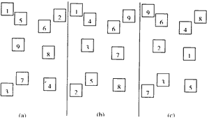
Figure 1. Examples of GCP distribution patterns. (a) Even coverage large to small, 9b) Even along-track left to right, (c) Even across-track center to edge.
1For the convenience of implementation, the order was defined as: top-left, top-right, bottom left and bottom-right as shown in Figure 1(a).
The even along-track (ALG) pattern cares only about across-track coordinate of GCPs (normally x-coordinate). The GCPs are sorted by this across-track coordinate to be ordered from left-to-right (L2R), right-to-left (R2L) center-to-edge (C2E) and edge-to-center (E2C). Figure 1(b) shows the example of the ALG_L2R pattern.
The even across-track (ACR) pattern can then be easily derived from ALG (90 degree rotation of ALG). The y-coordinate (along-track coordinate) or the GCPs determines the order of the GCPs. This pattern also consists of four sub-patterns: top-to-bottom (T2B), bottom-to-top (B2T), edge-to-center (E2C) and center-to-edge (C2E). Figure 1© shows the example of ACR_C2E pattern.
The total number of N GCPs are sorted according to each distribution pattern. The first n GCPs among the sorted GCPs are applied for the camera modeling and the rest N-n GCPs are used for the accuracy assessment (check points).by increasing n from 1 to N, we can analyze the performance of the camera model: its accuracy, convergence speed, and pattern-dependency.
It is known that the application of evenly-distributed GCPs to a camera model results in the best performance. The three patterns (COV_L2S, ALG_E2C, ACR_E2C) are expected to give the better camera modeling performance that the other seven patterns. We will, however, apply the all ten patterns to a camera model so that we can see the tolerance of a model to badly-distributed GCP patterns. The GCPs do have some errors inevitably and it is costly to obtain one accurate GCP. It is therefore better to use a camera model which is tolerant to GCP errors and requires the smallest number of GCPs.
3.Camera Models
The camera models can be categorized by the degree of assumptions and approximations. They are ranged from a fully abstract model such as the polynomial warping technique to a fully physical model which is too complex and practically impossible to be implemented analytically due to random variations of some physical parameters. The examples of assumptions are :
- Satellite orbit is circular or straight line in the scale of a scene
- Earth is flat, spherical or ellipsoidal
- Camera focal length or scan-line length are fixed
- Attitude of the satellite is fixed or a linear function of time, and so on
In this paper, we tested two camera models which are close to a full physical model. One is developed and published by Shin and Lee (Shin & Lee 1997, shin et al, 1998). It is based on Cartesian coordinate transformation from image coordinate to map coordinate and vice versa. This technique converts the raw image coordinates (column, row) to the ground coordinates (map projection) by modeling CCD alignment on focal plane, sensor scanning geometry, satellite orbit and attitude geometry, and Earth shape and rotation. The coordinate transform is performed by using a vector projection technique with axes rotation. The residual error sources after this systematic modeling are :
- Satellite position (along-track, across-track, radial)
- Satellite velocity (along-track,across-track, radial)
- Satellite attitude (pitch, roll, yaw)
The other model was developed by Toution (Toution 1983, 1995). The mathematical equation of the model is similar to the photogrammetric equation such as collinearity and coplanarity conditions. This model was integrated into a commercial photogrammetry and satellite image processing software, PCITM. PCI v.62 OrthoEngine software was used for the experiments.
4.Experiments
A SPOT-PAN image was selected as a test image. A total number of 22 GCPs (road crossings) were carefully selected from the test image and their image coordinates were determined with a sub-pixel precision. The ground truth data were collected by field measurements by using a differential GPS receiver giving a meter's accuracy (see Figure 2). The 22 GCPs were sorted according to each distribution pattern described in Section 2. The each ordered GCPs was applied to set the camera model and the rest were used as check points for the independent accuracy assessment.
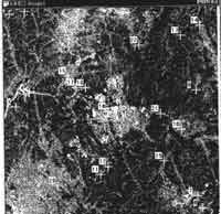
Figure 2. Test image : SPOT-PAN, viewing angle = -4.7deg.©CNES
Figure 3 shows results of the Shin & Lee's model. As described in Section 2, COV)L2S, ALG_E2C resulted in the fastest convergence to the final accuracy of about 10m (1 pixel). In this case, Shin & Lee's model can achieve the accuracy by using only 3~5 GCPs. Figure 4 shows the results of the PCI camera model. It shows that the PCI camera model requires than ten GCPs to achieve the final model accuracy.
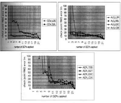
Figure 3: Performance of Shin & Lee's model
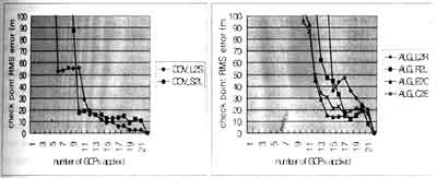
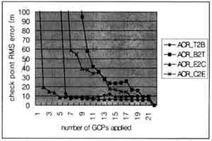
Figure 4: Performance of PCI model
5.Conclusions
This paper shows the performance of two different camera models with respect not only to the final accuracy but also to the number of GCPs required and their spatial distributions. The two camera models showed different characteristics according to the GCPs applied for modeling. It was also shown that as a camera model was implemented close to a physical model, it can achieve accurate results by using smaller number of GCPs. In addition, it not sensitive to the distribution patters of GCPs.
References
- Chang, D., J.Liu, Y. Jiang and H Li, 1990. Geometric correction with photographic model for satellite remote sensing images. SPIE Digital Image Processing and Visual communications Technologies in the Earth and Atmospheric Sciences, Vo. 1301,pp. 162-170.
- Moreno, J.F., 1993. A method for accurate geometric correction of NOAA AVHRR HRPT data. IEEE TGARS, 31 (1), pp. 204-226.
- Salamonowicz, P.H., 1986. Satellite orientation and position for geometric correction of scanner imagery, PE&RS, 52 (4), pp. 461-499.
- Shin, D. and Y.R. Lee, 1997. Geometric modeling and coordinate transformation of satellite-based linear pushbroom-type CCD camera images. J. Korean Society of Remote Sensing, 13(2), pp. 85-98. (written in Korean)
- Shin, D., Y.R. Lee and H.K. Lee, 1998, Precision correction of satellite-based linear pushbroom-type CCD camera images, J. Korean Society of Remote Sensing, 14(2), pp. 137-148. (written in Korean)
- Shin, D. and Y.R. Lee, 1998. Performance analysis on the geometric correction algorithms using GCPs - polynomial warping and full camera modeling. Processing of International Symposium of Remoe Sensing, Kwangju, Korea, pp. 252-256.
- Toutin, T., 1993. Analyse mathematique des possibilities cartographique du satellite SPOT, Memoire du diplome d'Etudes Aprofondies, Ecole Nationale des Sciences Geodesiques, Saint-Mande, France, p. 74.
- Toutin, T., 1995. Multi-source data fusion with an integrated and unified geometric modeling, EARSel Journal Advances in Remote Sensing, 4(2), pp. 118-129.