| GISdevelopment.net ---> AARS ---> ACRS 1999 ---> Poster Session 2 |
Correction of OCTS Sensor
Alignment
Toshiaki Hashimoto
Center for Environmental Remote Sensing (CEReS), Chiba University
1-33, Yayoi, Inage-Ku Chiba 263, JAPAN
TEL:(81)-43-290-3945 FAX:(81)-43-290-3857
http://www.gisdevelopment.net/aars/acrs/1999/ps2/hashi@ceres.cr.chiba-u.ac.jp
Center for Environmental Remote Sensing (CEReS), Chiba University
1-33, Yayoi, Inage-Ku Chiba 263, JAPAN
TEL:(81)-43-290-3945 FAX:(81)-43-290-3857
http://www.gisdevelopment.net/aars/acrs/1999/ps2/hashi@ceres.cr.chiba-u.ac.jp
Keywords: Sensor alignment, Collinearity
condition, ADEOS/OCTS
Abstract:
The alignments of ADEOS/OCTS were measured before the launch. But it was found out that the values of the alignments were changed after the launch, which resulted in the serious amount of geometric distortion. The alignments were corrected on the basis of photogrammetry using OCTS imagery and GCPs.
1. Introduction
The ADEOS(Advanced Earth Observing Satellite) was launched in August 1996 by NASDA (National Space Development Agency of Japan). The OCTS(Ocean Color and Temperature Scanner) on board the ADEOS spacecraft is an optical mechanical scanner with 12 channels and the spatial resolution of 680 m at nadir. It observed the Earth surface only in daytime. The geometric accuracy of the OCTS at initial check out was about 10 km on the ground. It was too terrible for some applications which needed high geometric accuracy like mosaicking, image composite, etc. The NASDA and some organization examined the reasons for such a terrible accuracy and ascertained three kinds of factors; 1) the bug of software for calculating satellite position, 2) the inadequacy of the algorithm for satellite attitude, 3) the change of alignments after the launch. In those factors, the bug for satellite position was fitted easily. The algorithm for satellite attitude was installed on the onboard computer. The raw attitude data were processed by the algorithm and transmitted to the ground. So the attitude data could be no longer corrected. But the only raw attitude data for first orbit each day in GMT were downlinked for housekeeping. Such raw data were processed with the new algorithm adopted for ADEOS-2/GLI (Global Imager). The subject of this paper is the correction of the alignments utilizing OCTS imagery on the basis of photogrammetry.
2. Scan geometry of OCTS
Figure 1 shows the optical pass from the focal plane to the ground. The orbital coordinates are introduced which is right handed where the flight and zenith direction correspond to x and z axis respectively. The OCTS has the tilt function by inclining the scanning mirror around y-axis (NASDA,1996). The vector a from the center of the focal plane to the scanning mirror is expressed as (1,0,0). If the tilt angle (t) is equal to zero, the normal vector of mirror 0will be ( cos(45° +e ), 0, sin(45° +e ) ), where e is the miss-inclination of mirror and equal to 14
milli-radians. When the scanning mirror is tilted by t and the scan angle is q ,
the normal vector of the mirror 1 is expressed as follows.
0will be ( cos(45° +e ), 0, sin(45° +e ) ), where e is the miss-inclination of mirror and equal to 14
milli-radians. When the scanning mirror is tilted by t and the scan angle is q ,
the normal vector of the mirror 1 is expressed as follows.
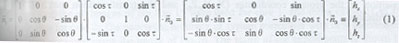
If the alignments of the scanning mirror ( a1, b1, l1) are considered, the normal vector of the mirror is expressed as=Q1•1.
The view vector reflected from the mirror is expressed as 1=
1= -2( ,)•. If the alignments of the sensor itself
to the platform (a2, b2, g2)
are considered, the view vector will be re-written as =Q2•1. In these equations, both
Q1 and Q2 are the rotation matrices around three
axes. The view vector is expressed by the components as follows.
-2( ,)•. If the alignments of the sensor itself
to the platform (a2, b2, g2)
are considered, the view vector will be re-written as =Q2•1. In these equations, both
Q1 and Q2 are the rotation matrices around three
axes. The view vector is expressed by the components as follows.
Figure 1 Scan geometry of OCTS (q=0)
3. Alignments to be determined
The effect of each alignment on the view vector is examined. The view vector without any alignment is expressed as1=(1-2hx2,
-2hxhy,-2hxhz. If each
alignment exist individually, the view vector is expressed as follows.
The differences of view vectors are expressed in Figure 2 by the error vectors on the image where each alignment has 0.001 radian independently. The calculation was performed on the equatorial region. Both the formula and the errors on the image proved that the a1.and a2 have the same effect on the image. Eventually the parameters (b1, g1) and (a2, b2, g2) are selected as the alignments to be determined and the value of a1 is fixed to the re-launch value in this work.
Figure 2 Errors on image raised by alignment error
4. Collinearity equation
The relationship between the satellite coordinates (x,y,z) and the ground coordinates (X,Y,Z) is expressed using the view vector in the satellite coordinates=( bx,
by, bz,) the satellite position in the ground
coordinates (X0,Y0,Z0) and the
transformation matrix (W) of both coordinates.
Finally, the collinearity equations can be introduced as follows (Hashimoto, 1997).
If the only alignments except other parameters like the satellite position, attitude and the ground coordinates are uncertain, they would be treated as unknown parameters. The collinearity equations are linearized by differentiating around unknown parameters.
5. Experiments and Results
The optimal alignments were corrected by the equation (6) utilizing GCPs. The OCTS images used here are LAC(Local Area Coverage) in Level 1B1 of which radiometric distortion and bands-to-bands registration error are corrected. The GCPs were collected manually from the images and TPC (Tactical Pilotage Chart) of 1:500,000.
The process needs the satellite position and attitude determined with high accuracy. The satellite position calculated by the bug-fixed software was verified with another independent determination using RIS (Retroreflector In Space) (Maeda,1996). The verification proved that the position could be determined in some ten meters. The satellite attitude data were not sufficiently correct as mentioned above. Only limited number of data could be processed with the new algorithm. In this research, two kinds of tactics were adopted; 1) to utilize a huge number of OCTS images without attitude data for mitigating attitude errors, 2) to utilize only OCTS images with the attitude data processed by new algorithm. Table 1 shows the OCTS images used in the experiment. In the table, ‘exist’ in attitude column means that the attitude data were processed with the new algorithm.
Table 1 OCTS images to be used
In the experiment, the all images of No.1 to 15 were used for case 1, and those of No.11 to 15 with attitude data for case 2. The geometric accuracy of system correction with new determined alignments was examined using the image of No.16. The result of the experiments is shown in Table 2. The result indicated that the geometric accuracy of system correction for case 1 was better than that for case 2. The alignments for case 1 might be suitable for geometric correction. But, if the new algorithm for GLI is correct, the alignments for case 2 would reflect the actual condition.
Table 2 Determined alignments and geometric accuracy of system
correction
case 1: 10 images without attitude and 5 images with attitude
case 2: 5 images with attitude
Vx : along track
Vx : cross track
In the exterior orientation using collinearity equation, if the only attitudes are treated as unknown parameters, the attitude would be estimated for minimizing the error distribution of GCPs by the system correction (Hashimoto, 1998). The estimated attitude was compared with those from raw data calculated by the new algorithm using the image of No.16. The alignments used here were those of case 2. The result is shown in Table 3. The estimated attitude was almost same as the observed one.
Table 3 Comparison of estimated and
observed attitude (deg.)
6. Conclusion
This paper described the method and some experiments for correcting the alignment error of OCTS on the basis of photogrammetry. Since the limited number of images with attitude data could be utilized, the images without attitude data were also used. The experiment indicated that the result by using many images would be proper for geometric correction, even if the attitude data could not be used. However, the correction using attitude data might reflect the actual condition. The experiences of ADEOS indicated the possibility of the change of the alignments after the launch. The technique in this paper will be utilized for ADEOS-2/GLI.
Reference
Abstract:
The alignments of ADEOS/OCTS were measured before the launch. But it was found out that the values of the alignments were changed after the launch, which resulted in the serious amount of geometric distortion. The alignments were corrected on the basis of photogrammetry using OCTS imagery and GCPs.
1. Introduction
The ADEOS(Advanced Earth Observing Satellite) was launched in August 1996 by NASDA (National Space Development Agency of Japan). The OCTS(Ocean Color and Temperature Scanner) on board the ADEOS spacecraft is an optical mechanical scanner with 12 channels and the spatial resolution of 680 m at nadir. It observed the Earth surface only in daytime. The geometric accuracy of the OCTS at initial check out was about 10 km on the ground. It was too terrible for some applications which needed high geometric accuracy like mosaicking, image composite, etc. The NASDA and some organization examined the reasons for such a terrible accuracy and ascertained three kinds of factors; 1) the bug of software for calculating satellite position, 2) the inadequacy of the algorithm for satellite attitude, 3) the change of alignments after the launch. In those factors, the bug for satellite position was fitted easily. The algorithm for satellite attitude was installed on the onboard computer. The raw attitude data were processed by the algorithm and transmitted to the ground. So the attitude data could be no longer corrected. But the only raw attitude data for first orbit each day in GMT were downlinked for housekeeping. Such raw data were processed with the new algorithm adopted for ADEOS-2/GLI (Global Imager). The subject of this paper is the correction of the alignments utilizing OCTS imagery on the basis of photogrammetry.
2. Scan geometry of OCTS
Figure 1 shows the optical pass from the focal plane to the ground. The orbital coordinates are introduced which is right handed where the flight and zenith direction correspond to x and z axis respectively. The OCTS has the tilt function by inclining the scanning mirror around y-axis (NASDA,1996). The vector a from the center of the focal plane to the scanning mirror is expressed as (1,0,0). If the tilt angle (t) is equal to zero, the normal vector of mirror
0will be ( cos(45° +e ), 0, sin(45° +e ) ), where e is the miss-inclination of mirror and equal to 14
milli-radians. When the scanning mirror is tilted by t and the scan angle is q ,
the normal vector of the mirror 1 is expressed as follows.
If the alignments of the scanning mirror ( a1, b1, l1) are considered, the normal vector of the mirror is expressed as
=Q1•1. The view vector reflected from the mirror is expressed as
1=-2( ,)•. If the alignments of the sensor itself
to the platform (a2, b2, g2)
are considered, the view vector will be re-written as =Q2•1. In these equations, both
Q1 and Q2 are the rotation matrices around three
axes. The view vector is expressed by the components as follows. Figure 1 Scan geometry of OCTS (q=0)
3. Alignments to be determined
The effect of each alignment on the view vector is examined. The view vector without any alignment is expressed as
1=(1-2hx2,
-2hxhy,-2hxhz. If each
alignment exist individually, the view vector is expressed as follows.
The differences of view vectors are expressed in Figure 2 by the error vectors on the image where each alignment has 0.001 radian independently. The calculation was performed on the equatorial region. Both the formula and the errors on the image proved that the a1.and a2 have the same effect on the image. Eventually the parameters (b1, g1) and (a2, b2, g2) are selected as the alignments to be determined and the value of a1 is fixed to the re-launch value in this work.
Figure 2 Errors on image raised by alignment error
4. Collinearity equation
The relationship between the satellite coordinates (x,y,z) and the ground coordinates (X,Y,Z) is expressed using the view vector in the satellite coordinates
=( bx,
by, bz,) the satellite position in the ground
coordinates (X0,Y0,Z0) and the
transformation matrix (W) of both coordinates. Finally, the collinearity equations can be introduced as follows (Hashimoto, 1997).
If the only alignments except other parameters like the satellite position, attitude and the ground coordinates are uncertain, they would be treated as unknown parameters. The collinearity equations are linearized by differentiating around unknown parameters.
5. Experiments and Results
The optimal alignments were corrected by the equation (6) utilizing GCPs. The OCTS images used here are LAC(Local Area Coverage) in Level 1B1 of which radiometric distortion and bands-to-bands registration error are corrected. The GCPs were collected manually from the images and TPC (Tactical Pilotage Chart) of 1:500,000.
The process needs the satellite position and attitude determined with high accuracy. The satellite position calculated by the bug-fixed software was verified with another independent determination using RIS (Retroreflector In Space) (Maeda,1996). The verification proved that the position could be determined in some ten meters. The satellite attitude data were not sufficiently correct as mentioned above. Only limited number of data could be processed with the new algorithm. In this research, two kinds of tactics were adopted; 1) to utilize a huge number of OCTS images without attitude data for mitigating attitude errors, 2) to utilize only OCTS images with the attitude data processed by new algorithm. Table 1 shows the OCTS images used in the experiment. In the table, ‘exist’ in attitude column means that the attitude data were processed with the new algorithm.
| No. | observation time (GMT) | tilt angle(deg) | No. of GCP | attitude | ||||
| 1 | 1996.11.29 02:39:56- | 0.00649 | 40 | no | ||||
| 2 | 1996.11.29 02:52:40- | -9.9912 | 38 | no | ||||
| 3 | 1996.12.30 02:13:31- | 0.00375 | 32 | no | ||||
| 4 | 1996.12.31 01:46:24- | 0.00375 | 28 | no | ||||
| 5 | 1997.04.14 02:54:26- | -9.4181 | 12 | no | ||||
| 6 | 1997.04.14 02:11:19- | 9.3175 | 11 | no | ||||
| 7 | 1997.04.16 02:41:00- | -9.4177 | 9 | no | ||||
| 8 | 1997.04.16 02:57:54- | 9.3161 | 7 | no | ||||
| 9 | 1997.04.25 01:58:28- | -9.4181 | 19 | no | ||||
| 10 | 1997.05.09 02:23:31- | -9.4179 | 15 | no | ||||
| 11 | 1996.12.12 01:51:04- | 0.00363 | 38 | exist | ||||
| 12 | 1996.12.12 02.23.31- | -9.9907 | 43 | exist | ||||
| 13 | 1996.12.16 01:45:55- | 0.00653 | 31 | exist | ||||
| 14 | 1997.05.16 02:37:25- | -94168 | 17 | exist | ||||
| 15 | 1997.06.17 01:57:45- | -9.4168 | 29 | exist | ||||
| 16 | 1997.06.01 02:04:55- | -9.3612 | 41 | exist | ||||
| ||||||||
In the experiment, the all images of No.1 to 15 were used for case 1, and those of No.11 to 15 with attitude data for case 2. The geometric accuracy of system correction with new determined alignments was examined using the image of No.16. The result of the experiments is shown in Table 2. The result indicated that the geometric accuracy of system correction for case 1 was better than that for case 2. The alignments for case 1 might be suitable for geometric correction. But, if the new algorithm for GLI is correct, the alignments for case 2 would reflect the actual condition.
| alignment | scanning mirror(sec) | OCTS sensor (deg) | error [pxl] | ||||||
| a1 | b1 | g1 | a2 | b2 | g2 | Vx | Vy | V | |
| Pre-Launch | -44.0 | -724.0 | 697.0 | -0.00170 | 0.00350 | 0.04390 | 7.58 | 4.42 | 8.775 |
| case 1 | -44.0 | -224.1 | 471.1 | -0.06405 | -0.06272 | 0.163852 | 0.81 | 1.12 | 1.378 |
| case 2 | -44.0 | -145.2 | 539.3 | -0.13395 | -0.06161 | 0.074248 | 2.44 | 1.11 | 2.683 |
case 1: 10 images without attitude and 5 images with attitude
case 2: 5 images with attitude
Vx : along track
Vx : cross track
In the exterior orientation using collinearity equation, if the only attitudes are treated as unknown parameters, the attitude would be estimated for minimizing the error distribution of GCPs by the system correction (Hashimoto, 1998). The estimated attitude was compared with those from raw data calculated by the new algorithm using the image of No.16. The alignments used here were those of case 2. The result is shown in Table 3. The estimated attitude was almost same as the observed one.
| scene | observation date | estimated | observed | ||||
| roll | pitch | yaw | roll | pitch | yaw | ||
| No.16 | '97.06.01 | 0.0458~-0.0064 | -0.0763 | -0.1017 | 0.048~-0.075 | -0.076 | -0.076 |
6. Conclusion
This paper described the method and some experiments for correcting the alignment error of OCTS on the basis of photogrammetry. Since the limited number of images with attitude data could be utilized, the images without attitude data were also used. The experiment indicated that the result by using many images would be proper for geometric correction, even if the attitude data could not be used. However, the correction using attitude data might reflect the actual condition. The experiences of ADEOS indicated the possibility of the change of the alignments after the launch. The technique in this paper will be utilized for ADEOS-2/GLI.
Reference
- Hashimoto, T., 1997, Precise Geometric Correction of ADEOS/OCTS
Imagery, Journal of JSPRS, Vol.36, No.5, pp42-51
- Hashimoto, T., 1998, The Estimation of Motion and Attitude of ADEOS Satellite utilizing the Principle of Exterior Orientation’, Journal of JSPRS, Vol.37, No.6, pp4-13
- Maeda, M., et al, 1996, Accuracy of Trajectory Determination and Prediction of ADEOS with RIS Experiment, Proc. of SPIE, Vol.3218, pp31-39
- NASDA, 1996, OCTS Algorithm Description