| GISdevelopment.net ---> AARS ---> ACRS 1999 ---> Poster Session 1 |
A practical model for
estimating the arable land change of China using remotely sensed
imagery
Zhongchao Shi 1
, Liu Haiqi 2 , Ryousuke Shibasaki
1
1 Center for Spatial Information Science and Institute of Industrial Science ,
the University of Tokyo
4-6-1 Komaba, Meguro-ku,Tokyo 153-8558 JAPAN
Tel. +81-3-5452-6413 Fax +81-3-5452-6414
Email : shizc@skl.iis.u-tokyo.ac.jp
2 Dept. of Development Planning, Ministry of Agriculture,
No.11 Nongzhanguan Nanli, Beijing, 100026, P.R.China
Tel/Fax:(010)64192552
E-Mail: Liuhaiqi@chnmail.com
Keywords : Arable land Change, Sampling,
Modeling1 Center for Spatial Information Science and Institute of Industrial Science ,
the University of Tokyo
4-6-1 Komaba, Meguro-ku,Tokyo 153-8558 JAPAN
Tel. +81-3-5452-6413 Fax +81-3-5452-6414
Email : shizc@skl.iis.u-tokyo.ac.jp
2 Dept. of Development Planning, Ministry of Agriculture,
No.11 Nongzhanguan Nanli, Beijing, 100026, P.R.China
Tel/Fax:(010)64192552
E-Mail: Liuhaiqi@chnmail.com
Abstract
A model which can estimate the nationwide arable land change based on number of sample data is proposed and described in this paper. Since the accuracy of the estimation is mainly depended on the number of samples and the sampling method, a method for selecting the optimum sampling number and optimum sampling location is proposed. The accuracy and efficiency of the proposed model was examined in China. The arable land change in totally 2550 counties were estimated from 238 samples(counties). By comparing the estimated results with the national statistic data, the mean error of the estimation is below 10 percent which satisfies the requirements for national arable land change investigation.
Introduction
To master the arable land and its change is very important for making national agricultural planning of a country. However, because of the limitation of budget, it is usually difficult and sometimes not necessary to use time series TM images which cover whole country for such a purpose. Generally, it can be solved by using so-called sampling technique, which can estimate the nationwide arable land change using just number of samples.
Basically, a sampling data based estimation method should satisfy following four requirements:
- Should be operational and feasible;
- With low cost;
- With high accuracy and reliability;
- Can estimate dynamically(high efficiency).
In this research, China was selected for testing. Because the national statistical reports of China are generally made from county level data, “county” is usually the smallest unit for statistical purpose. Hence, “county” will be used as the sampling unit in our discussion.
Statistical Arable Land Change Data
Figure 1 shows the distribution of statistical arable land changes of China in 1993 which includes 2550 units with an interval of 100 mu(mu is a widely used unit for present the amount of land, 1mu = 1/15 ha).Following units were not included :
- 75 county-level units in Tibet Autonomous Region because there are no available data from Tibet;
- Some municipal districts such as Beijing’s Eastern District and Western District because they are not arable lands;
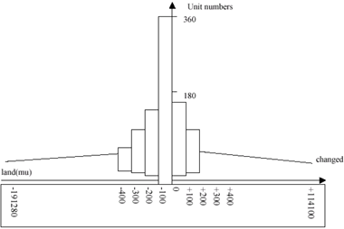
Fig.1 Distribution of arable land changes of China in 1993(statistical data).
Arable Land Change Estimation Model
Class number
In order to estimate the nation-wide arable land changes from limited sampling data, we have to at first classify the estimation units into several classes. Because the arable land changes involve quite a few random factors, the number of classes should be determined in order minimize the sampling rate. In this research, 6,8,10,12 classes were tested and 6 were found the best class number for estimation.
Class interval
According to figure 1, the accumulating value of squire root (f) of arable land changes can be calculated. The value is 653.4 which will be classified into 6 classes. Therefore, the interval of accumulation value of each class is 653.4/6 = 108.9. It is then easy to determine the start and end(boundary) values of each class as :
class 1: ( -¥, - 11800]
class 2: (- 11800, - 3800]
class 3: (- 3800, - 900]
class 4: (- 900, + 300]
class 5: (+ 300, + 3600]
class 6: (+ 3600, + ¥)
After the boundary value of each class has been determined, the numbers of units in each class can be countered easily from the figure 1. Here are the units in each of 6 classes :
class 1: ( -¥, - 11800] 115
class 2: (- 11800, - 3800] 223
class 3: (- 3800, - 900] 454
class 4: (- 900, + 300] 1187
class 5: (+ 300, + 3600] 419
class 6: (+ 3600, +¥) 143
sum 2541*
*As mentioned in section 2, 9 special units were removed from the total population of 2550 units because the change are very large.These 9 units should be investigated by inventory.
Determination of optimum sample number and location
According to the requirements of the project, the accuracy and reliability should be reached 90% and 95% respectively.
The optimum number of samples is able to be calculated according to following formula:
Where: n0, primary sampling size;
Nh, the figures of sampling units in class No. h ;
Sh, the square roots of the real variance of class No. h;
V, the figures of pre-assuming variance.
Because fpc=471/2541=18.5%>5%(fpc : finite population correction), finite population correction is needed. After FPC, the number of samples should be :
Based on the optimum allocation method, nh= [(Nh * Sh) /S(Nh*Sh)] * n , the 238 counties can be allocated into each class. The result is shown in Table 1.
| Class No. | 1 | 2 | 3 | 4 | 5 | 6 | sum |
| Nh (Total units ) |
115 | 223 | 454 | 1187 | 419 | 143 | 2541 |
| nh (Sampling units) |
97 | 23 | 17 | 16 | 17 | 68 | 238 |
Experiments and Discussions
Experimental results
The experiment was conducted using Landsat TM images. The sampling units of 202 counties under remote sensing investigation are chosen from Sichuan, Jiangsu, Heilongjiang, Guangdong, Gansu, Jiangxi, Shanxi Provinces and Xinjiang Autonomous Region. The total land area and total arable land area in selected region cover 370,000 square kilometers and 190 million mu respectively. In addition, 78 county level units (mainly distributed in class 1 and class 6) were selected for test. Therefore, total 280 units were used in our experiment. The estimation formula are shown below :
Where: y, estimated value of population average;
N, total unites of population;
yh, average value of stratum No. h.
Where: V(y), the variance value of population average;
Sh, variance value of stratum h;
nh, real sampling unites in stratum h.
Table 2 shows the estimated results calculated from eq. (3) and (4).
| class | Nh | Real nh | Sh | Average for sample y |
Y population | Standard Error of Y |
| 1 | 115 | 97 | 17941.97 | -2812.74 | -7358127.80 | 708410.92 |
| 2 | 223 | 26 | 4578.77 | |||
| 3 | 454 | 25 | 3534.51 | |||
| 4 | 1187 | 39 | 2446.92 | |||
| 5 | 419 | 19 | 3474.61 | |||
| 6 | 143 | 74 | 18679.89 | |||
| sum | 2541 | 280 |
Discussions
The errors occurred in this project came from two sources. One was the sampling error, which is S1=70.8 (sampling standard error); the other was the error in visual interpretation of satellite imagery (TM) . The visual interpretation work had been carried out for 3 years. The error in visual interpretation was about 5%. Hence the misinterpreted error is S2 = 7415000* 5% ˜371000 mu. Therefore, the general error (S) can be calculated as: S = square root (37.1*37.1+70.8*70.8) = 800,000 mu According to the relation between accuracy and reliability(Y±S*t), one can easy calculate accuracy according to the reliability requirement.
- Assuming the reliability requirement is 90% (t = 1.64),
then, the limiting error is t*S = 1.64*800,000= 1.31 million mu;
therefore, the accuracy of estimation is (741.4 - 131) / 741.5 = 82.5%. - Assuming the reliable interval is 85% (t = 1.46),
then, the limiting error is t*s = 1.46*80= 1.17 million mu;
So, the accuracy of this estimation is (741.4 - 117) / 741.5 = 84.2%.
It should be mentioned that the comparison of estimated results from remotely sensed imagery with the statistical data may not really obtain the accurate results. The major reason was that the original statistical data could not reflect the real situation. Taking Dongguan City of Guangdong Province as an example, the city lost several dozens thousands mu of arable land annually in recent years, but the decrease information was not reflected in its statistical datum. Some of the counties in Gansu Province reported their statistical datum which were of wide difference compared with the datum from remote sensing investigation. Moreover, the absolute value was same but the symbol was just opposite. Such problems can be only solved gradually with the deepening understanding of the population in the work and continuing improvement of class program.
Conclusions
This paper described a practical model for estimating the nationwide arable land change with some sampling data. The results of experiment shows that the professional technology method with integration of remote sensing technology and area sampling technology, is one of the most effective and economic methods for implementing the monitoring of the nationwide arable land resources changes.
The method and technology proposed in this model may be easily applied for monitoring or estimating other utilization status of the land, such as the planting area of main crops. In these cases, the sampling method may have to be modified.
In the future, we are going to test the model in other countries or regions. The possibility of applying proposed model in as macro investigation and management may also be investigated and discussed.
References
- William G. Cochran: Sampling Techniques, Third Edition, John Wiley & Sons,USA.1977
- Wigton W., Area frame sampling, documents for training course, USDA. 1979.
- Gallego,F.J., Delince,J., Area estimation by segment sampling. In Euro-Courses: Remote Sensing applied to Agricultural Statistics. JRC-ISPRA,ITALY,1993
- Meyor-Roux J., The ten years research and development plan for application of remote Sensing in Agricultural Statistics. Joint Research Center, EEC. publication No: JRC SP 1.87.pp39,24.