| GISdevelopment.net ---> AARS ---> ACRS 1999 ---> Poster Session 1 |
Integrating landscape Models
in Forest landscape Analyses using GIS: An Example in Taiwan
Li-Ta Hsu and Chi-Chuan
Cheng
Taiwan Forestry Research Institute, Council of Agriculture
53 Nanhai Rd., Taipei 100, China Taipei
Tel: (886)-2-2381-7107ex(203) Fax: (886)-2-2375-4216
E-mail: lita@serv.tfri.gov.tw China Taipei
Abstract Taiwan Forestry Research Institute, Council of Agriculture
53 Nanhai Rd., Taipei 100, China Taipei
Tel: (886)-2-2381-7107ex(203) Fax: (886)-2-2375-4216
E-mail: lita@serv.tfri.gov.tw China Taipei
Landscape monitoring is an important issue in landscape ecology and forest ecosystem management. This study used geographic information systems to integrate landscape models at different levels to analsyze landscape changes of the Liukuei ecosystem management area in Taiwan. Landscape maps of 1988 and 1996 wee derived from aerial photographs using digital photogrammetry. GIS programs wee used to calculate the landscape structure indices under different conditions. Markov models were then used to predict trends of landscape changes. Preliminary results indicate that natural processes and human interference both significantly affected the structures and land cover distributions of the study area. Without continued reforestation, natural forests would reclaim man-made stands gradually. Timber harvesting would not cause long-lasting effects on the landscape. Forestation, on the other hand, may induce landslides or create bare land. To address spatial variability of landscape changes, probabilistic models will be developed to examine factors associated with landscape changes and to predict probabilities of landscape changes spatially.
1. Introduction
Landscapes are assemblages of habitats, communities and land use types, and the spatial configuration of these landscape elements can be attributed to a combination of environmental correlates and human forces (Forman and Godron 1986). Landscapes are dynamic in structure, function, and spatial pattern. Therefore, monitoring landscape dynamics is a basic but important aspect of landscape ecology and ecosystem management. In human-dominated landscapes, changes in a landscape are often due to management practices. Therefore, protecting and preserving ecosystems requires an ability to predict the direct and indirect, temporal, and spatial effects of human activities (Costanza 1987).
Scientists often use landscape models to describe or explain landscape dynamics. Baker (1987) classified landscape models into three categories: (1) whole landscape models, (2) distributional landscape models, and (3) spatial landscape models. Whole landscape models focus on the value of a variable or several variables in a particular land area. Distributional landscape models emphasize changes in the distribution of land cover types. Spatial models, on the other hand, use the location and configuration of landscape elements in projecting change, and can explicitly produce maps of these changing spatial configurations.
There are many application examples of landscape models. For example, Turner (1989), Li (1990) and Dunning et al. (1992) used various landscape indices to measure landscape structures under different conditions. Markov models are probably the most commonly used distributional models. Burnham (1973) used a Markov simulation model to depict the intertemporal landscape changes in a southern Mississippi alluvial valley. Lindsay and Dunn (1979) applied a Markov model to project future distributional patterns of land uses in New Hampshire. With some modifications, distributional landscape models can be used to derive spatial landscape models. For example, Turner (1987) included neighborhood influences in deriving Markov transition probabilities to account for spatial variability. In recent years, probabilistic models such as logic models have become popular in modeling spatial landscape changes. For instance, Dale and others (1993) used a multi-nominal logic model to evaluate the deforestation pattern in Brazil. Hsu (1996) applied a binary logic model to examine factors affecting land use changes and to predict possible land use patterns in the future.
Landscape models at the three different levels are interrelated. Whole landscape models describe the characteristics of a certain landscape; distributional models examine or predict changes of landscape distribution over time; and spatial models determine where the changes might occur. However, those models were rarely integrated. Since landscape models are directly associated with spatial landscape patterns, the use of geographic information systems (GIS) can facilitate the integration of models at different levels. Therefore, the objective of this study is to proposed a framework for integrated landscape analysis. Various landscape indices, Markov models, and multinomial logic models are used to analyze the landscape changes in managed forest landscape in Taiwan. The results can provide useful information to decision-makers.
2. Material and methods
The 'Liukuei ecosystem management area' is a part of the Liukuei experimental forest of the Taiwan Forestry Research Institute (TFRI). The study area encompasses seven forest compartments, and covers about 2500 ha. Elevation in the area ranges from 300m to 1800m, and the topography is up-sloped from southwest to northeast. The Shan ping post and several nurseries are also located inside the area and are connected by service roads stretching throughout the area. Natural forests dominate 78% of the landscape, and man-made stands occupy the remaining 22%. Most of the man-made stands are conifers. Natural forests consist of many broadleaf tree species, and some are mixed with conifers. There are some cut areas due to timber harvesting. In addition, there are some non-forested areas such as grasslands or bare lands resulted from landslides.
Aerial photographs taken in 1988 and 1996 were used to generate landscape maps of the study area. Positive films of the photographs were scanned into digital images. The images were subsequently rectified as orthogonal images with accurate positioning. Image pairs were then displayed as stereographs on computer screens, where features on the landscape were delineated and digitized. As a result, two sets of vector files were created. For each land cover patch, its land cover type, area, and perimeter were recorded. The two maps were then overlid together using a geographic information system to identify land cover changes during the period.
The analytical procedures of this study include three steps. In the first step, various landscape indices was used to measure the structures of the landscape under different conditions. The landscape was classified into natural forests, man-made stands, bare lands, streams, roads and other man-made structures (such as buildings and nurseries). The following landscape indices were used to measure the structural characteristics of the landscape: (1) number of patches, (2) mean patch size, (3) largest patch index, (4) total edge, and (5) mean shape index. The formula for calculating shape index (SI) is:
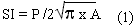
Where P is the perimeter and A is the area of a patch. The value of SI is equal is round-shaped, and the value increase if the shape of a patch becomes irregular.
In the second step. A first-order Markov model was used to examine the distributional changes of the landscape. The model can be expressed in matrix notation as:
Where nt is a column vector whose elements are the fraction of landscape in each of the m land cover types at time t, and P is an m x m matrix whose elements, Pij, represent the transition rate from one land cover type to each of the m land cover types during the time interval from to t+1. The transition probabilities were derived from the observed transitions occurred during the time interval. Maximum likelihood estimates of the transition probabilities were:
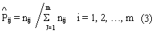
where nij are elements of the (m x m) 'transition matrix' representing the amount of transition from land cover type I to land cover type j. Several assumptions were made. First, the markov model was assumed to be a first-order process: that is, the state at time t+1 depends only on the state at time t and the transition probabilities, thus history previous to time t had no effect. Second, the transition probabilities were assumed to be stationary over time t had no effect. Second, the transition probabilities were assumed to be stationary over time. Then, Equation (2) was used project the subsequent landscape distributions. Under the assumption of stationary transition probabilities, iteration of equation (2) will ultimately culminate in an equilibrium distribution nt* which satisfies n*t+1 = Pn*t = n*t. The equilibrium distribution is the condition that the mangnitude of movements out of one land cover type is exactly equal to the movements into that land cover type. Elements of vector nt* represent the fraction of landscape in each of the m land cover types at the hypothetical equilibrium in the future.
While the Markov model predicts the distributional changes of the landscape in the future, it does not spatially predict where the changes might occur. Therefore, the third step of this study is to develop probabilistic models for predicting landscape changes spatially. To do so, multinomial models will be used to examine the factors contributing to landscape changes. Supposing landscape change from one land cover type to some other land cover type is dependent on Yi, which is a cumulative effect of several factors x1, x2, x3, … Yi can be written as:
If there are m cover types, then the probability of changing into land cover type I is:
Once the distributional changes predicted by the Markov model are determined, equation (5) can be used to predict where the changes might occur. The predicted landscape patterns can then be re-assessed by the landscape indices to evaluate the structural changes of the landscape.
3. Results and discussion
The landscape patterns of the Liukuei ecosystem management area are shown in Fig.1.

Fig 1 Landscape structures in 1988 and 1996 under different extents of interference.
The values of landscape indices under different conditions are compared in Table 1.
| Yr | Landscape index | Index value under cumulated effect | |||
| Original | Add streams | Add roads | Add stands | ||
| 1988 | Number of patches | 20 | 46 | 68 | 128 |
| Mean patch size (ha) | 122 | 53 | 36 | 19 | |
| Largest patch index (%) | 99 | 98 | 28 | 19 | |
| Total edge (km) | 7.1 | 66.4 | 136.0 | 176.4 | |
| Mean shape index | 1.40 | 4.00 | 4.30 | 3.16 | |
| 1996 | Number of patches | 29 | 64 | 82 | 159 |
| Mean patch size (ha) | 84 | 38 | 30 | 15 | |
| Largest patch index (%) | 99 | 98 | 28 | 20 | |
| Total edge (km) | 9.6 | 69.7 | 138.2 | 187.8 | |
| Mean shape index | 1.51 | 3.48 | 3.87 | 2.83 | |
The results indicate that forestation greatly increased the number of patches; streams significantly decreased the mean patch size; and road building affected the largest patch index the most. The total edge increased as the cumulated effect increased, but the effects of streams, road building and forestation did not differ by much. Streams and roads made the patches become irregular in shape. However, because man-made stands tend to be regular in shape, the mean shape indices decreased due to forestation. Comparing the index values in 1988 and 1996 indicates that forestation during the period increased the number of patches, decreased the mean patch size, and slightly increased the length of total edge. The mean shape index also decreased due to regular-shaped forestation. However, because natural forests reclaimed parts of the man-made stands, the largest patch index increased slightly.
| Transition from row to column | Man-made conifers | Man-made hardwoods | Mixed forests | Natural hardwoods | Bare lands | Cut areas | 1988 total |
| Man-made conifers | 384.3 0.841 |
3.1 0.007 |
13.6 0.036 |
50.6 0.111 |
5.4 0.012 |
0 0 |
457.0 1 |
| Man-made hardwoods | 1.5 0.017 |
48.3 0.563 |
1.4 0.016 |
34.6 0.403 |
0 0 |
0 0 |
85.7 1 |
| Mixed forest | 2.5 0.121 |
0.4 0.019 |
13.4 0.008 |
4.3 0.208 |
0.02 0.001 |
0 0 |
20.6 1 |
| Natural hardwoods | 35.1 0.119 |
60.9 0.034 |
13.97 0.008 |
1688.0 0.936 |
4.1 0.002 |
1.58 0.001 |
1803.7 1 |
| Bare lands | 1.0 0.051 |
0 0 |
0 0 |
13.7 0.727 |
4.2 0.222 |
0 0 |
18.9 1 |
| Cut areas | 12.25 0.248 |
14.65 0.297 |
10.4 0.211 |
11.7 0.237 |
0.4 0.007 |
0 0 | 49.4 1 |
| 1988 total | 436.6 | 127.4 | 52.7 | 1802.9 | 14.1 | 1.6 | 2435.3 |
Table 2 shows the Markovian transition matrix and transition probabilities of the observed landscape changes from 1988 to 1996. The landscape was classified into man-made conifers, man-made hardwoods, mixed forests, natural hardwoods, bare lands, and cut areas. The land cover distributions in 1988 and 1996 are summarized in the row and column total, respectively. The most apparent landscape change was the conversion of 95 ha of natural hardwoods into man-made stands. However, about 85 ha of man-made stands were reclaimed by natural hardwoods, too. Mixed forests also increased substantially. Cut areas, on the other hand, decreased dramatically because most of them were wither reforested or taken over by natural hardwoods. In the transition probability matrix, it shows that 11% of man-made conifers, 40% of man-made hardwoods, and 21% of mixed forests became natural hardwoods. Natural hardwoods also substantially reclaimed non-forested land. About 54% of cut areas wee reforested, and 45% of them were taken over by natural hardwoods, leaving less than 1% non-forested.
Using the land cover distribution in 1996 as the base year, subsequent land cover distributions were projected until the equilibrium condition was reached was reached. Table 3 compares the land cover distributions in 1988, 1996 and under the equilibrium.
| 1988 | 1996 | Equilibrium | |
| Man-made conifers | 457 | 437 | 311 |
| Man-made hardwoods | 86 | 127 | 155 |
| Mixed forests | 21 | 53 | 76 |
| Natural hardwoods | 1806 | 1803 | 1882 |
| Bare lands | 19 | 14 | 10 |
| Cut areas | 49 | 2 | 2 |
| Total area | 2436 | 2436 | 2436 |
The results suggest that the area of man-made conifers would decrease. However, continuing reforestation would increase the area of man-made hardwoods. The area of mixed forests would maintain at 76 ha. The area of natural hardwoods would increase. Non-forested cut areas would maintain at a very negligible size of 2 ha, and the area of bare lands would decrease. Results of long-term simulation show that it would take approximately 280 years to reach the hypothetical equilibrium.
4. Conclusions
Several conclusions can be drawn from this study. From the comparisons of landscape indices, it can be seen that natural processes and human activities both significantly affected the structure of the landscape. Streams did not increase the number of patches in the landscape by many, but it made the patches become irregular in shape. Moreover, because forest roads intersect with streams, streams and roads together divided the landscape into many small patches. Forestation, on the other hand, created many heterogeneous patches on the landscape. These results can provide forest managers useful information when planning for road building and forestation.
The results from Markov models indicate that natural recovery and management activities also significantly altered the land cover distributions. Without continued forestation, natural forests might eventually reclaim the man-made stands. Therefore, to plan for reforestation in the future, such processes should be taken into account. Even without man-made reforestation, natural forests would soon reclaim cut areas or non-forested lands. This implies that timber harvesting would not cause long-lasting effects to the landscape. However, landslides or bare lands appeared to be more likely to occur on man-made coniferous stands. Therefore, in areas vulnerable to natural disasters, extra care should be given when selecting forestation species.
This study demonstrates that using landscape indices and Markov models to assess landscape changes can provide useful information for management decision making. Landscape indices can be used to describe the structure of a landscape. While Markov models can be used to examine and predict distributional changes over time. However, these models do not explicitly predict where the changes might occur, neither do they explain the mechanisms underneath the changes. Therefore, the next step of this study is to develop spatially explicit models for predicting landscape changes. The integration of landscape indices. Markov models, and spatial model will enable a more thorough analysis of landscape changes.
Literatures cited
- Baker W.L. 1989. Areview of models of landscape change. Landscape Ecol 2(2): 111-33.
- Burnham B.O. 1973. Markov intertemporal land use simulation model. Southern J of Agri Econ 5:253-8.
- Costanza R. 1987. Social traps and environmental policy. BioSci37:407-12.
- Forman R.T.T. and M. Godron. 1986. Landscape ecology. New YorkL John Wiley and Sons. 619 p.
- Dale V.H., R.V. O'Nell, M. Pedlowski, and F. Southworth. 1993. Causes and effects of land-use change in central Rondonia, Brazil. Photogrammetric Engineering & Remote Sensing. 59(6): 997-1005.
- Dunning, J.B., B.J. Danielson and R.R. Pulliam 1992. Ecological processes that affect populations in comples landscapes. Oikos. 65:169-175.
- Hsu, L.T. 1996. Modeling land use change in human-dominated landscapes: a case study of urbanization in an Indiana watershed. West Lafayette, IN: Purdue University. 152p. PhD. Theses.
- Li, H. 1990. Spatio-temporal pattern analysis of managed forest landscapes: a simulation approach. Corvalis, OR: Oregon State University. 166p Ph.D. thesis.
- Lindsay B.E. and C.L. Dunn. 1979. Land use projections under alternative policies: a transition matrix approach. J Northeastern Agri Econ Council. 8(2): 87-99.
- Turner M.G. 1987. Spatial simulation landscape changes in Georgia: A comparison of 3 transition models. Landscape Ecol 1(1): 29-36.
- Turner, M.G. 1989. Landscape ecology: the effect of pattern on process. Annual Review of Ecological System. 20: 171-197.