| GISdevelopment.net ---> AARS ---> ACRS 1999 ---> Oceanography/Coastal Zone |
Mapping Ocean Oil Pollution
with ERS SAR Imagery
Jingxuan Lu, Hock Lim,
Mingquan Bao, Soo Chin Liew, and Leong Keong Kwoh
Centre for Remote Imaging, Sensing and Processing, National University of Singapore
Lower Kent Ridge Road, Singapore 119260, Republic of Singapore
Tel: (65) 874-6557, Fax: (65) 775-7717,
E-mail: crslujx@nus.edu.sg
Keyword: Oil slicks, detection and mapping,
occurrence intensity, ERS SARCentre for Remote Imaging, Sensing and Processing, National University of Singapore
Lower Kent Ridge Road, Singapore 119260, Republic of Singapore
Tel: (65) 874-6557, Fax: (65) 775-7717,
E-mail: crslujx@nus.edu.sg
Abstract
With a large coverage, short repeativity, day and night, and all weather capability, ERS SAR imagery has been proven to be a very effective tool for ocean oil spill monitoring. This paper discusses ocean oil pollution detection and mapping in the Southeast Asian waters by using ERS SAR data. Possible oil slicks are detected first from each image and a normalized average oil slick occurrence intensity is then computed after all the available multi-temporal scenes in an ERS frame have been studied. The scene in which most slicks have been detected in a frame is then selected for re-examination. All oil slicks detected on this image are then further classified into either high or low probability categories. A new normalised maximum oil slick occurrence intensity is computed for each of the total and high probability oil slicks. Spatial distribution maps of the average and worst oil pollution situation for the Southeast Asian waters are then derived.
Introduction
Oil pollution surveillance and mapping over a large ocean area has become easy with the launch of remote sensing satellites. Space-borne synthetic aperture radar (SAR) has, in particular, become a very popular tool for ocean oil slick monitoring due to its wide area coverage under all weather conditions, day and night. Some very successful examples of ERS SAR applications in marine oil spill detection have been documented, such as the near-real-time oil spill monitoring in Norway (Pedersen et al, 1995) and a successful anti-oil spill law prosecution case in Singapore (The Straits Times, 1997). In comparison with the already reported oil spill monitoring case studies by space-borne SAR data, spatial oil spill distribution mapping is still under exploited, especially over a large ocean area. A study on ocean oil spill statistics using the ERS SAR imagery in the Southeast Asian waters is reported (Lu et al, 1999). It is probably the first attempt in marine oil pollution mapping with satellite data over a large area. The present study first compiles the oil spill statistics extended over a much larger area in the Southeast Asia region, and then maps the worst oil pollution scenario in the region.
Oceans in the Southeast Asia are among the busiest in the world. Several major international shipping routes pass through this region connecting the Pacific Ocean to the Indian Ocean. Oil is transported mainly from the Middle East to Japan, United States and the Southeast Asian countries. This region is also rich itself in ocean oil deposits with intensive oil exploitation and inter-regional transport activities already in place. Large oil/gas fields can be found in the Gulf of Thailand, the South China Sea off the Brunei coast, and so on. Mapping the spatial distribution of oil pollution is the first critical step towards the protection of the region’s marine environment.
The study area lies between longitudes 90° E and 125° E, latitudes 10° S and 20° N. Three years of ERS-1/2 data from September 1995 to September 1998 archived in CRISP’s database was used. This includes a total of 657 frames with 5029 scenes. Since thousands of scenes would be required, use of high-resolution PRI products would impose a heavy load on the processing facility and also slow down the slick detection process. Thus, our in-house quick-look products were used instead. With 1000x1013 pixels per scene of 100km x 100km, this version of quick-look images is adequate for fast oil slick detection (ESA, 1998; Lu & Bao, 1999).
Oil Slick Detection and Mapping with ERS SAR
Oil films are very effective in damping wind-generated gravity-capillary short waves on the sea surface and hence appear dark against a brighter background on SAR images. The detectability depends on ocean surface wind speed. If wind speed is too low (typically below 2 to 3 m/s), the sea surface background does not have sufficient roughness to contrast with that of oil films. On the other hand, if wind speed is too high (typically above 15 m/s), oil slicks can be dispersed by the surface waves and disappear below the sea surface.
Not all-dark sea surface areas in SAR images are real oil slicks. Sea surface may also appear dark due to natural slicks, low wind, certain atmospheric and oceanic phenomena and other reasons. Contextual information such as the shapes and locations of the suspected oil slicks can also help to avoid false detection. The main challenge for successful oil slick detection depends on the exclusion of all those possible look-alike slicks. Examples of some typical signatures of oil slicks on ERS SAR images are shown in Figure 1.
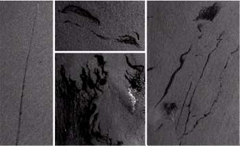
Figure 1. Examples of various oil slicks on ERS SAR images:
a). a long linear slick from a moving ship,
b). slicks from offshore oil rigs,
c). slicks probably from natural seepage, and
d). slicks along a major shipping route
Mapping of the average oil pollution distribution is performed in three steps. First, possible oil slicks in each scene are visually identified and discriminated against other look-alike features. Next, these identified oil slicks are further classified into one of the three categories based on their shapes, namely linear, curved and patchy. In addition, the size of each slick is also estimated and grouped into one of four categories, namely “<1km”, “1-5km”, “5-10km”, and "³10km".Lastly, a normalized average oil slick occurrence intensity is then computed for each frame after all the available scenes in this frame have been examined. This pollution index is defined to be the average slick number detected each time per 10,000 km2 sea surface. For a given frame, it is expressed by the equation:
where Ni is the total number of slicks detected in the i-th scene, fsea is the sea surface fraction of the frame, and fi is the scene fraction of the i-th scene.
Mapping of the worst oil pollution distribution is based on the above steps. The scene on which most slicks have been detected in a frame is then selected for re-examination. All detected oil slicks on this image are further classified into either high or low probability ones. A similar normalised oil slick index for either total or high probability slicks can be calculated for this frame as:
where N is the detected slick number of the scene for any of the total, high & low probability slicks, fsea is the sea surface fraction of the frame, and f is the scene fraction. These steps are repeated until all the included ERS frames have been completed so that the spatial distribution of oil pollution distribution in the region can be derived.
Spatial Distribution of the Average Oil Slick Occurrence Intensity
The overall statistical result for the average oil slick occurrence intensity is summarised in Table 1. A total of 10988 oil slicks have been detected in 2292 scenes, representing 45.6% of the total scenes studied. Spatially speaking, over 80% of the total study area had been once polluted at an intensity of at least one slick per 10,000 km2 of sea surface area during the study period. Linear and patchy slicks have an almost equal frequency (45%) with curved ones much lower (10%). More than 10% of the oil slicks are over 10 km in size and over a quarter below 1 km in size, while about 60% of the total detected slicks fall in the range of 1-10 km.
Table 1. Statistical results of the detected oil slicks in the Southeast Asian waters during the period of September 1995 to September 1998.
| Detected slicks | Number | Percentage (%) | |
| Total | 10988 | 100.0 | |
| Slick types | Linear | 5045 | 45.9 |
| Curved | 1175 | 10.7 | |
| Patchy | 4768 | 43.4 | |
| Slick sizes | ³10km | 1338 | 12.2 |
| 5-10km | 1824 | 16.6 | |
| 1-5km | 4695 | 42.7 | |
| <1km | 3131 | 28.5 | |
| Total scenes | 5029 | 100.0 | |
| Total frames | 657 | 100.0 | |
| Polluted scenes | 2292 | 45.6 | |
| Polluted frames | 552 | 84.0 | |
The normalised slick intensity is summarised in Table 2. The averaged oil pollution intensity over the whole study area is 2.7 with the highest of 28.8. The normalised slick intensity is then used to compile the spatial distribution map of the average ocean oil slick occurrence intensity in this region (Figure 2).
Table 2. Statistical results of the normalized average oil slick occurrence intensity in the Southeast Asian waters during the period of September 1995 to September 1998.
| Intensity | Total | Slick type | Slick size (km) | |||||
| Linear | Curved | Patchy | ³10 | 5-10 | 1-5 | <1 | ||
| Maximum | 28.8 | 16.7 | 6.0 | 13.3 | 10.6 | 5.5 | 13.3 | 8.4 |
| Average | 2.7 | 1.2 | 0.3 | 1.2 | 0.3 | 0.4 | 1.1 | 0.8 |
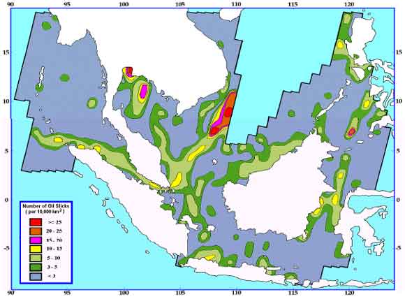
Figure 2. Spatial distribution map of the average oil pollution occurrence intensity in the Southeast Asian waters.
Spatial Distribution of the Maximum Oil Slick Occurrence Intensity
The overall statistical result for the worst polluted scenes is summarised in Table 3. A total of 5019 oil slicks have been detected, of which the high and low probability oil slicks take about one half each, i.e. 52% and 48%, respectively. The normalised oil slick occurrence intensity is summarised in Table 4. The averaged value of the normalized total oil slick occurrence intensity over the whole study area is 8.9 with the highest of 60.0. These values are more than twice of the above normalized average oil slick occurrence intensity. The averaged value of the normalized high probability oil slick occurrence intensity over the whole study area is 4.6 with the highest of 43.1. Figure 3 and Figure 4 are the spatial distribution maps of the normalised oil slick occurrence intensity for the total detected slicks and those high probability ones in the region, respectively.
Table 3. Statistical results of the detected oil slicks of those worst polluted scenes in the Southeast Asian waters during the period of September 1995 to September 1998.
| Detected slicks | Number | Percentage (%) |
| Total | 5019 | 100.0 |
| High probability | 2621 | 52.2 |
| Low probability | 2398 | 47.8 |
Table 4. Statistical results of the normalized oil slick occurrence intensity of those worst polluted scenes in the Southeast Asian waters during the period of September 1995 to September 1998.
| Intensity | Total | High | Low |
| Maximum | 60.0 | 43.1 | 47.6 |
| Average | 8.9 | 4.6 | 4.2 |
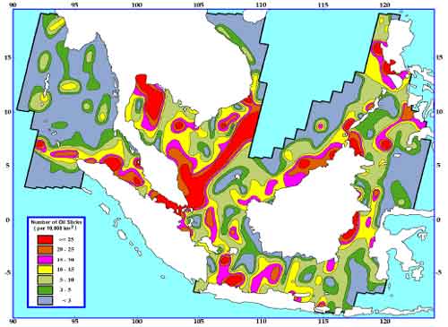
Figure 3. Spatial distribution map of the oil pollution occurrence intensity of the total detected oil slicks on those worst polluted images in the Southeast Asian waters.
Figure 4. Spatial distribution map of the oil pollution occurrence intensity of the high probability oil slicks on those worst polluted images in the Southeast Asian waters.
Conclusions
The average and maximum oil pollution intensity maps clearly show that areas of intense oil pollution correlate very well with the major shipping routes. The main shipping routes with high incidences of oil spills include the Straits of Malacca, the Singapore-Java route, the numerous routes crossing the South China Sea, the Singapore-Bangkok route, the Jakarta-Manila route, the Manila-Lombok route. The most polluted areas are found in the South China Sea and the Gulf of Thailand. The heavily polluted area in the South China Sea is believed due to deliberate oil discharges from ships due to its alignment with shipping routes. A mosaic of 4 worst polluted scenes in the South China Sea off the East Coast of the Malay Peninsula is show in Figure 5. Slicks on the mosaic are located along the main shipping route and have a clear orientation.
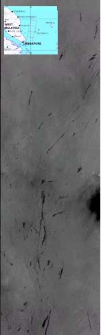
Figure 5. A mosaic of four worst polluted scenes in the South China Sea off the East Coast of the Malay Peninsula.
This study shows that it is feasible and very efficient to map oil pollution over a very wide ocean area using ERS SAR imagery. A study with the co-operative efforts of the many ground stations covering various parts of the world, a global map of ocean oil pollution intensity can be obtained. The results could greatly improve our awareness towards our ocean environment and help us locate those potentially vulnerable areas for future surveillance and protection.
References
- Pedersen, J.P., Seljelv, L.G., Strøm, G.D., Follum, O.A., Andersen, J.H., Wahl, T., and Skøelv, Å., 1995. Oil Spill Detection by Use of ERS SAR Data - From R & D towards Pre-operational Early Warning Detection Service. Proc. of the 2nd ERS applications workshop, London, UK, 6-8 Dec 1995, pp:181-185.
- Cracking an Oily Case with some Help from Above: Satellite Picture Helped to Finger Oil-spill Ship. The Straits Times, 19 Jan 1997, Singapore.
- Lu, J., H. Lim, S. C. Liew, M. Bao and L. K. Kwoh, 1999. Oil pollution statistics in Southeast Asian waters compiled from ERS synthetic aperture radar imagery. Earth Observation Quarterly, Nr. 61, Feb. 1999, pp: 13-17.
- Oil Pollution Monitoring. ESA BR-128, vol. 1, 1998.
- Lu, J. and Bao, M., 1999. A study on oil spill detection using different ERS SAR resolution data. Proc. of Int. Geoscience and Remote Sensing Symposium, 28 June -2 July 1999, Hamburg, Germany, pp: 806-808.