| GISdevelopment.net ---> AARS ---> ACRS 1999 ---> Oceanography/Coastal Zone |
The Sea Level Anomalies in
China Seas from Satellite Altimeter Data
Haiying Wang, Lintao Liu,
Houtse Hsu, Guangyun Wang
Lab of Dynamic Geodesy, Institute of Geodesy & Geophysics,
Chinese Academy of Sciences, Wuhan 430077
Keywords: Satellite Altimeter, Sea Level
Anomaly, China SeasLab of Dynamic Geodesy, Institute of Geodesy & Geophysics,
Chinese Academy of Sciences, Wuhan 430077
Abstract
In this paper, the collinear method is used to determine mean sea surface heights and its variations in the region of China Seas with Topex/Poseidon and ERS-1 altimeter data during the period from October of 1992 to June of 1997. After having done the corrections of T/P altimeter instrument bias and the geophysical environment corrections of tide, ionosphere, wet and dry troposphere, sea-state bias and inverse barometry, we find that the rising rates vary in different regions. Compared with the global annual sea level rising rate (+2.1 ± 1.3mm/yr), the annual rising rate in Yellow Sea, East Sea and South China Sea is +3.44 ± 0.61 mm/yr, +3.12 ± 0.47 mm/yr, and –1.41 ± 0.48 mm/yr, respectively. From the sea level anomalies, it can be seen clearly that the influence of El Nino in 1993, 1994, and 1997-1998 is greatest in South China Sea, less in East Sea and least in Yellow Sea. In addition to normal FFT spectrum analysis, a new wavelet analysis of WAPS was also used to the sea level anomalies. The results show that the annual period is stationary in all interest regions, but the semi-annual and seasonal periods have some degree of period drift. In addition, we also found there exists a clear two months period in all three regions whose mechanism is still to be explored.
The tidal gauge measurements are usually used in the traditional analysis of sea level variations but ones often have to face the problem of even locations of tidal gauges and the deformation of crust where tidal gauges locate. Thanks to the new remote sensor of satellite altimeter which was actually started with the launch of Skylab in 1978 by NASA, the world-wide sea surface heights in all-weathers can be measured in short time, such as 10 days, 17 days or 35 days. The altimeter missions of Geos-3 (NASA, 1975), Seasat (NASA, 1978) and Geosat (US Navy, 1985) prove the unique role of satellite altimeter in aspects of the determination of ocean circulation, sea surface topography and geoid undulations, and the improvement of gravity geopotential model. Because of one order improvement in radial orbit error, better corrections of atmospheric medium (ionosphere and troposphere), and the better oceanic tidal model, the unprecedented accuracy of ERS-1 (ESA, 1991), Topex/ Poseidon (NASA/CNES, 1992), ERS-2 (ESA, 1995), or GFO (US Navy, 1998) satellite altimeter is achieved. The altimeter data, which directly measure satellite-to-sea distances or indirectly measure sea levels, are very important to research in geodesy, geophysics as well as oceanography. As a result, a new generation of satellite altimeter, such as Envisat (ESA, 2005), Jason (NASA, 2005) will be launched in the first decade of coming 21st century.
In this paper, Topex/Poseidon and ERS-1 altimeter data during the period from October of 1992 to June of 1997 are used to determine mean sea surface heights and its variations in the region of China Seas with the collinear method. After having done the corrections of T/P altimeter instrument bias and geophysical environment corrections of tide, ionosphere, wet and dry troposphere, sea-state bias and inverse barometry, we get the variations of sea surface heights in the China Seas and vicinity. Besides common harmonic analysis and FFT analysis, a new wavelet analysis of WAPS is also used to the variations of mean sea level. The results in the region of Yellow Sea, East Sea and South China Sea will be discussed in detail.
Altimeter Data Processing
Topex/Poseidon (T/P) and ERS-1 satellite altimeter data used in this paper are from the AVISO CD ROMs of corrected Sea Surface Heights (SSH) (AVISO, 1996). The time span of altimeter data covers from October 3rd, 1992 to June 12, 1998. The interest regions are China Yellow Sea (119° - 126° E, 33° - 37° N), East Sea (120° - 127° E, 26° - 33° N) and South China Sea (110° - 119° E, 14° - 23° N). The period of each T/P cycle is 10 days and the period of each ERS-1 cycle is 35 days. The length of each 1-second corrected SSH is 32 bytes which contains 6 parameters, i.e., latitude, longitude, time, the corrected SSH, a reference mean sea surface (OSUMSS95) and inverse barometer correction. The corrected SSHs have been corrected by the EM bias, tidal corrections, wet and dry troposphere corrections, ionosphere correction, radial orbit corrections, gravity center correction of instrument, and inverse barometer effect. The correction models used for corrected SSH are shown in Table 1. For T/P altimeter data, the accuracy of the 1- second corrected SSH is estimated about 5 cm (Fu, et al., 1994), while the precision of T/P radial orbit is about 3-4 cm due to the higher precision tracking system of SLR and DORIS, the higher altitude of satellite orbit, the improvement of non-conservative force model and Earth gravity model, and the satellite-to-satellite tracking technique of GPS (Tapley, et al., 1994). Therefore, no orbit corrections are calculated for T/P, i.e., T/P orbits are taken as the reference level and the radial orbit error of ERS-1 is reduced by fitting the ERS-1 orbits into the more precise T/P orbits with dual-satellite crossover adjustment. This provides the accuracy of ERS-1 orbit similar to that of T/P orbit: 2 cm (Le Traon, et al., 1995). Moreover, the ERS-1 bias and any long-wavelength errors are simultaneously estimated with orbit error. This provides homogeneous precision between ERS-1 and T/P altimeter data. Because the repeating periods of T/P and ERS-1 cycles are different, ERS-1 altimeter data are also assimilated to T/P altimeter data, i.e., the repeating period of the assimilated altimeter data is 10 days. The assimilated altimeter data contain whole T/P data in a 10-day cycle and a part of ERS-1 data of a 35-day cycle. In addition, the Topex altimeter range calibration corrections (http://obs.wff.nasa.gov) derived from on-broad internal instrument measurements [Hayne et al., 1994] are also used. There is a shortening of the range over 1992-1998 of 0.52 ± 0.9 mm/yr. However, much of the error due to random noise still exists. So if an approximate smoothing is made, the accuracy can be increased to about 2-3 cm (Cheney, et al., 1994; Mitchum, 1994). In this paper, an average of measurements is interpolated every 10 seconds along each T/P and ERS-1 track with a criterion of three times of standard deviation. This smoothing scheme reduces the altimeter noise by approximately a factor of 2 while preserving sufficient horizontal resolution.
Table 1. The environmental corrections used in the corrected sea surface heights
| corrections | Topex/Poseidon | ERS-1 | |
| Orbit | NASA JGM3 orbits | D-PAF orbits | |
| Geophysical Corrections |
Dry troposphere Wet troposphere Ionosphere Inverse barometer |
from ECMWF from TMR radiometer TOPEX:from dual frequency altimeter range POSEIDON:from DORIS from ECMWF |
from ECMWF from ATSR-M radiometer BENT model from ECMWF |
| Sea State Bias (EM Bias) | BM4 formula | -5.5% of significant wave height | |
| Tides | Ocean tide & loading tide Solid tide Pole tide |
CSR 3.0 Cartwright and Taylor model (1971) applied |
CSR 3.0 Cartwright & Edden model with Wahr’s radial correction not applied |
Results and Discussion
Figure 1 shows the variations of sea surface heights in China Yellow Sea, East China Sea and South China Sea from October of 1992 to June of 1998, respectively. A traditional harmonic analysis is applied to the variations of sea surface heights to determine the amplitude and phase of annual, semi- annual, seasonal and two-month period, respectively. A FFT analysis is also applied. The results of harmonic and FFT analysis are shown in Table 2. The amplitudes of annual period are largest in all of the three interest regions which means the contributions of annual period are greatest and can be seen easily in Figure 1. The smoothing curves without marks in Figure 1 indicate the sum of the contributions of annual and semi-annual period. The straight lines indicate the secular contributions of the variations in the sea surface heights. However, the contributions of semi-annual and seasonal period are different in three interest regions. In Yellow Sea the contribution of seasonal is greater than that of semi-annual, in South Sea the case is inverse, and in East Sea there is equivalent between the contribution of semi-annual and that of seasonal. What we are surprised is that an about two month period exists obviously in all three interest regions and its amplitude exceeds that of semi-annual and seasonal in Yellow Sea and East Sea. This phoneme is proved in the following wavelet analysis.
Fig. 1 The variations of sea surface heights
(
 indicates China Yellow Sea, indicates
China East Sea, X indicates South China Sea)
indicates China Yellow Sea, indicates
China East Sea, X indicates South China Sea)
Table 2. The amplitudes of the variations in sea surface heights using the harmonic and FFT analysis (unit: mm)
|
| ||||||||
| Period | Annual | Semi-annual | Seasonal | 60 days | ||||
| Harmonic | FFT | Harmonic | FFT | Harmonic | FFT | Harmonic | FFT | |
|
| ||||||||
| Yellow Sea | 81.02 | 63.36 | 15.25 | 11.77 | 28.41 | 36.29 | 45.33 | 37.11 |
| East Sea | 75.75 | 59.31 | 18.19 | 12.39 | 14.70 | 12.19 | 69.76 | 52.06 |
| South Sea | 54.83 | 11.91 | 22.04 | 19.05 | 9.00 | 7.50 | 10.93 | 9.90 |
|
| ||||||||
The anomalies in the variations of sea surface heights, i.e., sea level anomalies or variations of mean sea level, are what we focus on. Figure 2 shows the sea level anomalies by removing the contributions of secular, annual and semi-annual periods from the variations of sea surface heights, and low-pass filtering with a bandwidth of seasonal, i.e., 90 days to reduce the effects of high frequency. The dash line in Figure 2 indicates the ENSO index (Nino3) from NCEP of NOAA (http://http://www.cpc.ncep.noaa.gov/). From the comparison between the sea level anomalies and ENSO index, we found that the effect of ENSO on the sea level anomalies in South China Sea is the largest. Furthermore, the 1997-1998 El Nino, which is the greatest in history, has the biggest effect, and causes a maximum negative anomaly of 30 mm. The sea level anomalies and the ENSO index almost become asymmetrical relation in South China Sea, while the respond of sea level anomalies on El Nino in China Yellow Sea and East Sea is an oscillation process and has an about six-month delay.
Figure 2 Sea level anomalies and its relationship to ENSO index
The solution of secular term from the variations of sea surface heights should be carefully carried out. The large contribution from the harmonic cycles should be removed first, such as annual cycle and semi-annual cycle. Then a low-pass filtering should be applied to reduce the random noise. Finally, the secular term can be obtained by linearly fitting the low-pass filtered residuals. The estimated sea level rise in China Yellow Sea, East Sea and South China Sea during 1992– 1998 is +3.44 ± 0.61 mm/yr, +3.12 ± 0.47 mm/yr and –1.41 ± 0.48 mm/yr, respectively. Compared with the global sea level rise +2.1 ± 1.3 mm/yr from 4 years T/P altimeter data (Nerem, et al., 1997), we found the sea level rises vary in different regions of China Seas, and there is a very strong correlation with the strongest El Nino of 1997-1998. For example, the rate in South China sea becomes negative due to the 199-1998 El Nino, while the rates in China yellow Sea and East Sea are almost the same because they are closing to each other.
In recent years, the Wavelet analysis becomes a very useful method in data processing because of its multi-resolution analysis. Wavelet analysis works as a mathematical micro-magnifying glass, so it has a better resolution in local frequency domain as well as in local space domain than common FFT analysis. Here we introduce a new wavelet analysis technique named ‘wavelet amplitude-period spectrum’ (WAPS) rather than the common wavelet energy spectrum analysis (Liu, 1999). WAPS can help to express and reveal instantaneous amplitudes and instantaneous frequencies of quasi-periodical signals. The definition of WAPS is as follows: if the real part of Morlet wavelet is chosen as a wavelet basis y(t), i.e.,
From the definition of WAPS, we prove that when a cosine signal
 reaches its limits ± A at
t=t0+nT/2, the WAPS of f(t) also reaches its limits ± A at the
locate (a=w0 T , b=t0
+nT/2). Therefore, when a signal consists of several cosine (sine)
periodical components, the limits and their locations of WAPS can
definitely determine the amplitude, period and phase of each periodical
component. It should be noted that the periods and amplitudes of
components in most actual signals usually change. Sometimes when the
periods of two components are close to each other, there is a coupling so
as difficult to separate the two components. In this case, the scales and
locations of the limits in WAPS of the signal will affect each other. Of
course, when the amplitudes and periods of components are stationary, and
the periods of each component are discrete large enough, the scale and
locations of the limits in WAPS can definitely express and reveal
instantaneous amplitudes and instantaneous frequencies of each periodical
component.
reaches its limits ± A at
t=t0+nT/2, the WAPS of f(t) also reaches its limits ± A at the
locate (a=w0 T , b=t0
+nT/2). Therefore, when a signal consists of several cosine (sine)
periodical components, the limits and their locations of WAPS can
definitely determine the amplitude, period and phase of each periodical
component. It should be noted that the periods and amplitudes of
components in most actual signals usually change. Sometimes when the
periods of two components are close to each other, there is a coupling so
as difficult to separate the two components. In this case, the scales and
locations of the limits in WAPS of the signal will affect each other. Of
course, when the amplitudes and periods of components are stationary, and
the periods of each component are discrete large enough, the scale and
locations of the limits in WAPS can definitely express and reveal
instantaneous amplitudes and instantaneous frequencies of each periodical
component. Figure 3 shows the results of WAPS analysis on the variations of sea surface heights in China Yellow Sea, East and South China Sea, respectively. The following results can be obtained:
- The annual periods in all three interest regions are very stable, and their amplitudes are also biggest. However during the 1997- 1998 El Nino which is strongest in history, the annual periods and its amplitudes in all three regions drift and change to a certain extent.
- The semi-annual and seasonal periods and their amplitudes in different regions are unstable. In South China Sea, the semi-annual term is stronger and more stable than the seasonal, but during 1997-1998 El Nino an inverse case occurred (i.e., the seasonal is stronger than the semi-annual), and the seasonal was weak and even disappear during the 1993 and 1994 El Nino. In China East Sea, the situation is almost the same as that in South China Sea. However in China Yellow Sea, the seasonal is stronger and more stable than the semi-annual.
- An about 60-day period is obviously found in three regions with different strength. The 60-day period in East Sea is the strongest, weaker in Yellow Sea, weakest in South Sea. The simulative mechanism of 60-day period is still to be investigated.
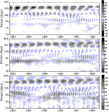
Figure 3 The results of WAPS analysis on the variation of sea surface heights (scale bar: mm) (bottom: China Yellow Sea; middle: China East Sea; top: South China Sea.
Conclusions
The sea surface heights derived from T/P and ERS-1 altimeter data have been compared with the measurements of tidal gauge in WOCE. It shows the T/P altimeter data have a good agreement with the measurements of tidal gauge. The correlation between T/P altimeter data and tidal measurements during 1992-1998 is 0.98 with rms of 2.1 cm. This indicates that it is reliable and feasible to study the mean sea level and its variations by using satellite altimeter data.
The estimated sea level rise in China Yellow Sea, East Sea and South China Sea from October 1992 to June 1998 is +3.44 ± 0.61 mm/yr, +3.12 ± 0.47 mm/yr and –1.41 ± 0.48 mm/yr, respectively. However, because the time interval of altimeter data in this paper spans only five and half years, the influence of inter-annual and decade periods of sea level variations can not be determined. With longer time series and higher precision of altimeter data, such as a proposed T/P follow-on satellite, named ‘Jason’, it is possible to provide an accurate long-term sea level rise rate from satellite altimeter data.
The contributions of each period vary in different regions, but the annual contribution is the largest one in all regions and its period are fairly stable too. Ranking the contributions of each period from descending order will result in: annual ® two months ®seasonal ® semi-annual in Yellow Sea; annual ®two months ®semi-annual ®seasonal in East Sea; annual ®semi-annual ®two months ® seasonal in South China Sea. It is explained that the sea level changes in Yellow Sea are mostly influenced by seasonal variation of Spring, Summer, Autumn and Winter, while in South China Sea they are mostly influenced by Sun’s crossing the equator twice a year.
The effect of El Nino on sea level anomalies is biggest in South China Sea, less in East Sea, and least in Yellow Sea. Since the duration of 1997-1998 El Nino lasted almost a year, 1997-1998 El Nino mainly affects the semi-annual period even the annual period and causes them drifted, weaken or disappeared. Because the 1993 El Nino and 1994 El Nino lasted not more than half year, they mainly affect the seasonal period and cause them drifted, weaken or disappeared.
Acknowledgement
This work is supported by a project of National Sciences Foundation Committee of China (code No. 49634140). We are grateful to CLS Space Oceanography Division, France provide us the CORSSH data.
References
- AVISO User Handbook: Corrected Sea Surface Heights (CORSSHs). AVI-NT-011-311-CN, Edition 2.0, 1996
- Cheney, R., L. Miller, R. Agreen, et al., TOPEX/POSEIDON: the 2-cm solution, J. Geophys. Res., 99(C12): 24555-24563, 1994
- Fu, L.L., E.J. Christensen, M. Lefebvre et al., TOPEX/ POSEIDON mission overview, J. Geophys. Res., 99(C12): 24369-24381, 1994
- Hayne, G.S., D.W. Hancock, and C.L. Purdy, TOPEX altimeter range stability estimation from calibration mode data, TOPEX/ POSEIDON Research News, 3, 18-22,1994
- Liu, L.T., Basic wavelet theory and its applications in geosciences, Ph.D dissertation, Institute of Geodesy and Geophysics, Chinese Academy of Sciences, 1999
- Mitchum, G., Comparison of TOPEX sea surface heights and tide gauge sea level, J. Geophys. Res., 99(C12): 24541-24553, 1994
- Nerem et al.: Improved determination of global mean sea level variations using Topex/Poseidon altimeter data, Geophys. Res. Lett., 24 (11), 1331-1334, 1997
- Tapley B D, Nerem R S, Shum C K, et al. Precision orbit determination for Topex/Poseidon altimetry. J. Geophys. Res., 1994, 99(C12), 24383-24404
- Le Traon P Y, Stum J, Dorandeu J, et al. Using Topex/Poseidon data to enhance ERS-1 orbit, J. Atm. Ocean. Tech., 1995, 12, 24619-24631
- Wagner C A, Cheney R E. Global sea level change from satellite alitmetry, J. Geophys. Res., 1992, 97(C10): 15607-15615