| GISdevelopment.net ---> AARS ---> ACRS 1999 ---> Mapping From Space |
Improved "Cloud-Free"
Multi-Scene Mosaics of Spot Images
Min Li, Soo Chin Liew,
Leong Keong Kwoh and Hock Lim
Centre for Remote Imaging Sensing and Processing
National University of Singapore, Lower Kent Ridge Road, Singapore 119260
Tel: (65) 8746586 Fax: (65)7757717
E-Mail: crslimin@nus.edu.sg
Centre for Remote Imaging Sensing and Processing
National University of Singapore, Lower Kent Ridge Road, Singapore 119260
Tel: (65) 8746586 Fax: (65)7757717
E-Mail: crslimin@nus.edu.sg
Keywords: Cloud-free, Balance, Rank, Mosaic
Abstract
An algorithm is described for automatic generation of "cloud-free" scenes from many SPOT images over a given region. It is commonly known that remote sensing using optical sensors often suffers from the presence of cloud covers, especially over the humid tropical regions. This problem can be partially overcome by acquisition of multiple images within a specified time interval over a given region. It is assumed that the land covers do not change within this time interval. By mosaicking the cloud-free areas in the set of images, a reasonably cloud-free composite image can be made. In this paper, we explicate the approach for generating "cloud-free" multi-scene mosaics of SPOT images.
1. Introduction
Optical remote sensing always encounters the problem of cloud covers, especially over the tropical areas. However, if multiple images acquired at different time over a given region are available, then it is possible to generate a reasonably cloud-free composite scene by mosaicking the cloud-free areas in the set of images. We have previously reported an operational algorithm for generating such cloud-free mosaics from multispectral images acquired by the SPOT satellites (Liew, 1998). In this algorithm, an intensity-thresholding method was used to identify the best cloud-free and non-shadow pixel among the pixels from the multiple images of a given region. In this intensity-thresholding method, bright pixels of land surfaces or buildings could be mistaken as cloud pixels, and they were ranked inferior than the cloud shadow pixels. Hence, these bright pixels were often replaced by cloud shadows. In areas covered by thin clouds or haze (especially over low-albedo vegetated areas or water surfaces), the hazy pixels would be selected instead of the cloud free pixels which were mistaken as cloud shadows.
In this paper, an improved algorithm for generating cloud-free multi-scene mosaics of SPOT images is reported. This improved algorithm avoids the pitfalls of the previous algorithm by making use of band ratios to classify the non-cloud and non-shadow pixels into one of three broad classes: water, vegetation or buildings. The intensity-based ranking rules were then modified accordingly to favour the selection of these "good pixels" instead of cloud shadows or thin clouds.
2. Description of the Algorithm
Figure 1 shows a schematic diagram of the operational system for generating cloud-free mosaics from SPOT images. With minimal modification, this system can also be used to generate cloud-free mosaics from optical images acquired by other satellites (e.g. Landsat-TM).
Fig. 1: A schematic diagram of the cloud-free mosaic generating system
2.1 Input Images
The inputs to the system are SPOT multispectral images of the same region acquired within a specified time interval, pre-processed to level 2A or 2B. The images are also co-registered before being fed into the system. The SPOT HRV sensor, when operating in the multispectral mode, captures data in three spectral bands, i.e. the green band (Band 1, 0.50 to 0.59 µ m), red band (Band 2, 0.61 to 0.68 µ m) and near-infrared band (Band 3, 0.79 to 0.89 µ m). In the conventional false-colour display of a SPOT multispectral image, band 3, band 2, and band 1 are assigned to the red, green and blue display channels respectively.
2.2 Radiometric Balancing
The radiometric balancing procedure assumes a Lambertian surface. It only makes a correction for differences in sensor gains, solar incidence angles and solar flux between the acquired scenes and no attempt has been made to have a correction for atmospheric effects. Suppose that a set of N images is available for a given scene. For each band-k of the set of images, the pixel values are radiometrically balanced with respect to each other according to
where the additional subscript n (n = 0, 1, 2, ..., N-1) is an index identifying the individual image within the set of N images, Rk,n is the pixel digital number of the radiometrically balanced image, DNk,n is the pixel digital number of the input image, gg,n is the sensor amplifier gain. Fk,n is the extra-terrestrial solar flux, qn is the solar elevation angle, ck is a multiplicative constant (same for all n) which stretches the balanced digital numbers to fill the range from 0 to 255. The above equation assumes that the ground reflectance did not change during the time interval within which these N images were acquired.
2.3 Pre-processing
The radiometric balancing procedure makes no attempt to correct for atmospheric effects. After radiometric balancing, the brightness of pixels at the same location from two different scenes will be a little different due to the atmospheric effects, especially in low-albedo vegetated areas. The pre-processing procedure tries to make a balance between the scenes for the differences caused mainly by atmospheric effects. After radiometric balancing, one image from the set of images is chosen as the reference image. For each band, the pixel values of all other images in the same set are adjusted according to
P=Eref+(S-E)*sref /
s (2)
where P is the output pixel value, S is the input pixel value, Eref is the mean pixel value of a selected area of interest from the reference image, E is the mean pixel value of a selected area of interest from the image to be balanced, sref is the standard deviation of the selected area of interest from the reference image, s is the standard deviation of the selected area of interest from the image to be balanced.
2.4 Pixel Ranking
The pixel ranking procedure uses the pixel intensity (weighted average of the three band pixel values) and some suitably chosen band ratios to rank the pixels in order of "cloudiness" and "shadowiness" according to some predefined ranking criteria. In this procedure, a shadow intensity threshold Ts and a cloud intensity threshold Tc are determined from the intensity histogram. The pixel ranking procedure uses these shadow and cloud thresholds to rank the pixels in order of "cloudiness" and "shadowiness". Each of the non-cloud and non-shadow pixels in the images is classified into one of four broad classes based on the band ratios: vegetation, building, water and others.
For each image n from the set of N acquired images, each pixel at a location (i, j) is assigned a rank rn(i, j) based on the pixel intensity Yn(i, j) and the brightness of the three display channels Rn(i, j), Gn(i, j) and Bn(i, j) according to the following rules:
(i) For Ts£(Ym, Yn) £ Tc, if Ym> Yn and class="building", then rm<rn;
(ii) For (Ym, Yn) £Tc if Ym < Yn and class="vegetation", then rm<rn ;
(iii) For Ym , Yn<Ts , if Ym > Yn and class="water", then rm < rn;
(iv) For Ts £(Ym , Yn)£Tc , if Ym<Yn and class="others", then rm<rn ;
(v) If (Ts £ Ym £TC,) and (Yn> TC or Yn<TC) and class="others", then rm<rn;
(vi) For YM, Yn<TC , if YM> Yn and class="others", then rm <rn;
(vii) If Ym<Ts and Yn > Tc then rm<rn;
(viii) For Ym , Yn > Tc , if Ym < Yn and class="others", then rm<rn;
In this scheme, pixels with lower rank values of r n are more superior and are more likely to be selected. Pixels with intensities falling between the shadow and cloud thresholds are the most superior, and are regarded as the "good pixels". Where no good pixels are available, the "shadow pixels" are preferred over the "cloud pixels". Where all pixels at a given location are "shadow pixels", the brightest shadow pixels will be chosen. In locations where all pixels have been classified as "cloud pixels", the darkest cloud pixels will be selected.
After ranking the pixels, the rank-r index map n r (i, j) representing the index n of the image with rank r at the pixel location (i, j) can be generated. In our algorithm, only the rank-1 and rank-2 index maps are generated and kept for use in generating the cloud-free mosaics.
2.5 Merging of Sub-Images
In this procedure, the rank-1 and rank-2 index maps are used to merge the multi-scenes from the same set of images. If the pixel at a given location has been classified as "vegetation pixel", the pixels from the rank-1 image and the rank-2 image at that location are averaged together in order to avoid sudden spatial discontinuities in the final mosaicked image. Otherwise, the pixels from the rank-1 image are used.
2.6 Selection and Masking of the Base Image
In order to get better visual effects it is desirable to have as many pixels as possible in the neighbourhood of a given location to come from the same scene. In this procedure, the image which was deemed to have the lowest cloud coverage by visual inspection is chosen to be the base image. Cloud and shadow thresholds are then applied to this base image to delineate the cloud shadows and the cloud covered areas. In the next step of mosaic generation, only the delineated cloud and shadow areas will be replaced with pixels from the merged image generated from the previous step.
2.7 Mosaic Generation
The final mosaic is composed from the merged images and the base image. These images are geo-referenced to a base map using control points. The mosaic generation transforms the coordinates of the pixels in the merged images and the base image into map coordinates and put the pixels onto the final image map.
3. Results and Conclusions
The cloud-free mosaicking algorithm has been tested successfully by using about 50 SPOT scenes over Singapore and the whole Johor State (Malaysia). Figure 2 shows a mosaic of cloudy SPOT images of the test area. Figure 3 is a "cloud-free" multi-scene mosaic of SPOT images generated using the algorithm presented here. The result shows that approximately 90 percent of the mosaic are free from clouds or shadows.
In this paper, we have presented an improved algorithm for generating cloud-free multiple scene mosaics of SPOT images. As in the previous method, this method uses the shadow and cloud thresholds to rank the pixels in order of "cloudiness" and "shadowiness". However, in this improved version, band ratios have been used to classify the pixels into a few broad land cover classes and the ranking rules have been modified to avoid mistaking low-albedo vegetation or water as cloud shadows and high-albedo open land or buildings as clouds.
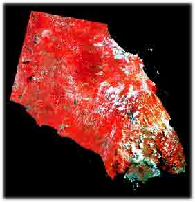
Fig. 2: Mosaic of cloudy SPOT images of Singapore and Southern Peninsular Malaysia Images with the lowest cloud coverage have been chosen to generate this mosaic.
(SPOT images . CNES, acquired and processed by CRISP, reproduced under licence from SPOT IMAGE)
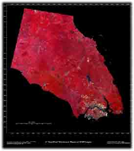
Fig. 3: Multi-scene cloud-free mosaic of Singapore and Southern Peninsular Malaysia generated using 48 SPOT scenes.
(SPOT images . CNES, acquired and processed by CRISP, reproduced under licence from SPOT IMAGE)
References from Other Literature:
Abstract
An algorithm is described for automatic generation of "cloud-free" scenes from many SPOT images over a given region. It is commonly known that remote sensing using optical sensors often suffers from the presence of cloud covers, especially over the humid tropical regions. This problem can be partially overcome by acquisition of multiple images within a specified time interval over a given region. It is assumed that the land covers do not change within this time interval. By mosaicking the cloud-free areas in the set of images, a reasonably cloud-free composite image can be made. In this paper, we explicate the approach for generating "cloud-free" multi-scene mosaics of SPOT images.
1. Introduction
Optical remote sensing always encounters the problem of cloud covers, especially over the tropical areas. However, if multiple images acquired at different time over a given region are available, then it is possible to generate a reasonably cloud-free composite scene by mosaicking the cloud-free areas in the set of images. We have previously reported an operational algorithm for generating such cloud-free mosaics from multispectral images acquired by the SPOT satellites (Liew, 1998). In this algorithm, an intensity-thresholding method was used to identify the best cloud-free and non-shadow pixel among the pixels from the multiple images of a given region. In this intensity-thresholding method, bright pixels of land surfaces or buildings could be mistaken as cloud pixels, and they were ranked inferior than the cloud shadow pixels. Hence, these bright pixels were often replaced by cloud shadows. In areas covered by thin clouds or haze (especially over low-albedo vegetated areas or water surfaces), the hazy pixels would be selected instead of the cloud free pixels which were mistaken as cloud shadows.
In this paper, an improved algorithm for generating cloud-free multi-scene mosaics of SPOT images is reported. This improved algorithm avoids the pitfalls of the previous algorithm by making use of band ratios to classify the non-cloud and non-shadow pixels into one of three broad classes: water, vegetation or buildings. The intensity-based ranking rules were then modified accordingly to favour the selection of these "good pixels" instead of cloud shadows or thin clouds.
2. Description of the Algorithm
Figure 1 shows a schematic diagram of the operational system for generating cloud-free mosaics from SPOT images. With minimal modification, this system can also be used to generate cloud-free mosaics from optical images acquired by other satellites (e.g. Landsat-TM).
Fig. 1: A schematic diagram of the cloud-free mosaic generating system
2.1 Input Images
The inputs to the system are SPOT multispectral images of the same region acquired within a specified time interval, pre-processed to level 2A or 2B. The images are also co-registered before being fed into the system. The SPOT HRV sensor, when operating in the multispectral mode, captures data in three spectral bands, i.e. the green band (Band 1, 0.50 to 0.59 µ m), red band (Band 2, 0.61 to 0.68 µ m) and near-infrared band (Band 3, 0.79 to 0.89 µ m). In the conventional false-colour display of a SPOT multispectral image, band 3, band 2, and band 1 are assigned to the red, green and blue display channels respectively.
2.2 Radiometric Balancing
The radiometric balancing procedure assumes a Lambertian surface. It only makes a correction for differences in sensor gains, solar incidence angles and solar flux between the acquired scenes and no attempt has been made to have a correction for atmospheric effects. Suppose that a set of N images is available for a given scene. For each band-k of the set of images, the pixel values are radiometrically balanced with respect to each other according to
where the additional subscript n (n = 0, 1, 2, ..., N-1) is an index identifying the individual image within the set of N images, Rk,n is the pixel digital number of the radiometrically balanced image, DNk,n is the pixel digital number of the input image, gg,n is the sensor amplifier gain. Fk,n is the extra-terrestrial solar flux, qn is the solar elevation angle, ck is a multiplicative constant (same for all n) which stretches the balanced digital numbers to fill the range from 0 to 255. The above equation assumes that the ground reflectance did not change during the time interval within which these N images were acquired.
2.3 Pre-processing
The radiometric balancing procedure makes no attempt to correct for atmospheric effects. After radiometric balancing, the brightness of pixels at the same location from two different scenes will be a little different due to the atmospheric effects, especially in low-albedo vegetated areas. The pre-processing procedure tries to make a balance between the scenes for the differences caused mainly by atmospheric effects. After radiometric balancing, one image from the set of images is chosen as the reference image. For each band, the pixel values of all other images in the same set are adjusted according to
where P is the output pixel value, S is the input pixel value, Eref is the mean pixel value of a selected area of interest from the reference image, E is the mean pixel value of a selected area of interest from the image to be balanced, sref is the standard deviation of the selected area of interest from the reference image, s is the standard deviation of the selected area of interest from the image to be balanced.
2.4 Pixel Ranking
The pixel ranking procedure uses the pixel intensity (weighted average of the three band pixel values) and some suitably chosen band ratios to rank the pixels in order of "cloudiness" and "shadowiness" according to some predefined ranking criteria. In this procedure, a shadow intensity threshold Ts and a cloud intensity threshold Tc are determined from the intensity histogram. The pixel ranking procedure uses these shadow and cloud thresholds to rank the pixels in order of "cloudiness" and "shadowiness". Each of the non-cloud and non-shadow pixels in the images is classified into one of four broad classes based on the band ratios: vegetation, building, water and others.
For each image n from the set of N acquired images, each pixel at a location (i, j) is assigned a rank rn(i, j) based on the pixel intensity Yn(i, j) and the brightness of the three display channels Rn(i, j), Gn(i, j) and Bn(i, j) according to the following rules:
(i) For Ts£(Ym, Yn) £ Tc, if Ym> Yn and class="building", then rm<rn;
(ii) For (Ym, Yn) £Tc if Ym < Yn and class="vegetation", then rm<rn ;
(iii) For Ym , Yn<Ts , if Ym > Yn and class="water", then rm < rn;
(iv) For Ts £(Ym , Yn)£Tc , if Ym<Yn and class="others", then rm<rn ;
(v) If (Ts £ Ym £TC,) and (Yn> TC or Yn<TC) and class="others", then rm<rn;
(vi) For YM, Yn<TC , if YM> Yn and class="others", then rm <rn;
(vii) If Ym<Ts and Yn > Tc then rm<rn;
(viii) For Ym , Yn > Tc , if Ym < Yn and class="others", then rm<rn;
In this scheme, pixels with lower rank values of r n are more superior and are more likely to be selected. Pixels with intensities falling between the shadow and cloud thresholds are the most superior, and are regarded as the "good pixels". Where no good pixels are available, the "shadow pixels" are preferred over the "cloud pixels". Where all pixels at a given location are "shadow pixels", the brightest shadow pixels will be chosen. In locations where all pixels have been classified as "cloud pixels", the darkest cloud pixels will be selected.
After ranking the pixels, the rank-r index map n r (i, j) representing the index n of the image with rank r at the pixel location (i, j) can be generated. In our algorithm, only the rank-1 and rank-2 index maps are generated and kept for use in generating the cloud-free mosaics.
2.5 Merging of Sub-Images
In this procedure, the rank-1 and rank-2 index maps are used to merge the multi-scenes from the same set of images. If the pixel at a given location has been classified as "vegetation pixel", the pixels from the rank-1 image and the rank-2 image at that location are averaged together in order to avoid sudden spatial discontinuities in the final mosaicked image. Otherwise, the pixels from the rank-1 image are used.
2.6 Selection and Masking of the Base Image
In order to get better visual effects it is desirable to have as many pixels as possible in the neighbourhood of a given location to come from the same scene. In this procedure, the image which was deemed to have the lowest cloud coverage by visual inspection is chosen to be the base image. Cloud and shadow thresholds are then applied to this base image to delineate the cloud shadows and the cloud covered areas. In the next step of mosaic generation, only the delineated cloud and shadow areas will be replaced with pixels from the merged image generated from the previous step.
2.7 Mosaic Generation
The final mosaic is composed from the merged images and the base image. These images are geo-referenced to a base map using control points. The mosaic generation transforms the coordinates of the pixels in the merged images and the base image into map coordinates and put the pixels onto the final image map.
3. Results and Conclusions
The cloud-free mosaicking algorithm has been tested successfully by using about 50 SPOT scenes over Singapore and the whole Johor State (Malaysia). Figure 2 shows a mosaic of cloudy SPOT images of the test area. Figure 3 is a "cloud-free" multi-scene mosaic of SPOT images generated using the algorithm presented here. The result shows that approximately 90 percent of the mosaic are free from clouds or shadows.
In this paper, we have presented an improved algorithm for generating cloud-free multiple scene mosaics of SPOT images. As in the previous method, this method uses the shadow and cloud thresholds to rank the pixels in order of "cloudiness" and "shadowiness". However, in this improved version, band ratios have been used to classify the pixels into a few broad land cover classes and the ranking rules have been modified to avoid mistaking low-albedo vegetation or water as cloud shadows and high-albedo open land or buildings as clouds.
Fig. 2: Mosaic of cloudy SPOT images of Singapore and Southern Peninsular Malaysia Images with the lowest cloud coverage have been chosen to generate this mosaic.
(SPOT images . CNES, acquired and processed by CRISP, reproduced under licence from SPOT IMAGE)
Fig. 3: Multi-scene cloud-free mosaic of Singapore and Southern Peninsular Malaysia generated using 48 SPOT scenes.
(SPOT images . CNES, acquired and processed by CRISP, reproduced under licence from SPOT IMAGE)
References from Other Literature:
- Liew, S. C., Li, M., Kwoh, L. K., Chen, P. and Lim H. (1998), "Cloud-free" multi-scene mosaics of SPOT images. Proc. 1998 International Geoscience and Remote Sensing Symposium, Vol. 2, 1083-1085.