| GISdevelopment.net ---> AARS ---> ACRS 1999 ---> Land Use |
Supervised Classification of
Multispectral Satellite Images using Fuzzy Logic and Neural Network
Somying Promcharoen and
Yuttapong Rangsanseri
Department of Telecommunications Engineering, Faculty of Engineering
King Mongkut's Institutte of Technology Ladkrabang, Bangkok 10520
Tel: (66-2)326-9967, Fax: (66-2)326-9086,
E-mail: kryutta@kmitl.ac.th
Suwit Ongsomwang and Jirawan Jaruppat
Forest Research Office, Royal Forest Department
Chatuchak, Bangkok 10900
Tel: (66-2)940-5737,
E-mail: suwit@forest.go.th
THAILAND
Keywords: Fuzzy Logic, Neural Network,
Supervised Classification, Multi-spectral Image.
Abstract: In this paper we present an algorithm based on fuzzy logic and neural network for supervised classification of multi-spectral satellite images. To deal with fuzzy information, gray level values of each multi-bath pixel are converted into three linguistic properties. This provides feature vectors in term of fuzzy membership values to the input of a neural network while the output vector is defined in term of membership value of each category. Experiments were carried out using Landsat-Tm data and the results are compared to those obtained by the conventional neural network classifier.
1. Introduction
The multi-layer perceptron (MLP) using the back-propagation (BP) algorithm is the convectional neural network model widely used in the supervised classification of multispectral satellite image data. By using training pixels, the network can be trained adaptively by updating its connection weights. The desired output is clamped to two state values: 1 to 0 (state 1 for 'belong to' and state 0 for 'not belong to' a category) (McCelland, 1986; Rangsanseri, 1998). But in real world, an input feature may possess a property with a certain degree of confidence or a pattern may belong to more than one category.
To deal with this fuzzy classification problem, an algorithm based on fuzzy logic and neural network was proposed. This algorithm is capable of handling input features (gray level values in each multi-band pixel), present in the three linguistic properties corresponding to each input feature, to the input of a neural network while assign output membership values of each category lying in the range [0,1] instead of 0 or 1 to the output vectors (desired output vector). This provides scope for increases its robustness in tackling imprecise input specification and allows modeling of fuzzy data which may belong to more than one category.
The MLP model and BP algorithm is described in the first section. In the following section the fuzzy sets, the pattern representation in linguistic form and the membership of output vector are described. Then we explain the fuzzy extension to BP algorithm. Finally, the experimental results using Landsat-TM data are given and compared to those obtained by the conventional neural network classifier.
2. MLP Model and BP Algorithm
The MLP model using the BP algorithm consists of sets of nodes arranged in multiple layers called input, output, and hidden layers. Only the nodes of two different consecutive layers are connected by weights, but there is no connection among the nodes in the same layer. For all nodes , except the input layers nodes, the total input of each node is the sum of weighted outputs of the nodes in the previous layer. Each node is activated with the input to the node and the activation function of the node. The input and output of the node I (except for the input layer) in a MLP model according to the BP algorithm (Pao, 1989) is :
The sum in eq. (1) is over all nodes j is the previous layer. The Sigmoid function (McCelland, 1986) given in eq. (3) is used to determine the output state.
f(Xi)=1/(1+exp(-Xi)) (3)
where Wij is the weight of the connection from node i to node j, bi the numerical value called bias, and f() the activation function.
The BP algorithm is designed to reduce an error between the actual output and the desired output of the network in a gradient descent manner. The summed squared error (SSE) is defined as:
Where p indexes the all training patterns and i indexes the output nodes of the network. Opi and tpi denote the actual output and the desired output of node i, respectively, when the input vector p is applied to the network.
A set of representative input and output patterns is selected to train the network. The connection weight Wij are adjusted when each pattern is presented. All the patterns are repeatedly presented to the network until the SSE function is minimized. Application of the gradient descent method (Bendiktsson, 1990) yields the following iterative weight update rule:
DWij(n+1)=h(diOi)+aDWij(n) (5)
where Wij is the weight of the connection from node i to j, h the learning factor, a the momentum factor, and di the node error. For output node i, di is then given by:
di =(ti-Oi)Oi(1-Oi) (6)
The node error at an arbitrary hidden node i is:
3. Fuzzy Logic
In conventional neural network classifier, an element r either 'belong to' or 'not belong to' a given category A is expressed as:
Using fuzzy logic, the element r belonging to the universe R, may be assigned a grade of membership with the membership function mA( r ) to a fuzzy set A is defined as:
A={(mA(r),r)}, rÎR, mA( r )Î [0,1]
3.1 Pattern representation in linguistic form
Each input feature Fj be expressed in terms of membership values to each of the three linguistic properties: low, medium, and high. Therefore an n-band-pattern will be represented as a 3n-dimension
vector.
will be represented as a 3n-dimension
vector.
We use the membership function (Pal, 1992) with range [0,1] and r ÎRn which is defined as eq. (9) to convert Fj to its three-dimensional form which is given by eq. (8).
where l is the radius of the p functuion, c the central point, and || . || the Euclidean norm.
Note that, the membership value decreases when its distance from the central point c(||r-c||) increase. It is maximum (p=1) when the pattern r lies at the central point c of a category (||r-c||=0).
Let Fjmax and Fjmin are the upper and lower bounds of the feature Fj in all L pattern points. Then the three linguistic property sets are defined as :
where fdenom is the parameter controlling the extent of overlapping. The overlapping structure of the p functions for the three linguistic properties is shown in Figure 1.
Figure 1: Overlapping structure of the p functions for the three linguistic properties.
3.2 Category membership of output vector
We use the Beta membership function to define the desired output of the network (this allows the desired output, lies in the interval [0,1], not clamped to only state 1 (belong to a category) or state 0 (not belong to a category).
The Beta membership function of the ith pattern to the kth category, with range [0,1] are defined as:
Where Zik: the weight distance from the ith input pattern to the center of the Kth
category
to the center of the Kth
category
b and p: the denominational and the exponential fuzzy generators which control the amount of fuzziness.
Mk: the mean of the mean of the numerical input patterns for the kth category
Fij: the value of the jth component of the ith pattern point.
Note that when the distance is 0 the membership value is 1 (maximum) and when the distance is infinite the membership value is 0 (minimum).
4. Fuzzy Extension to BP Algorithm
The fuzzy extension to BP algorithm consists of two steps. The first step is the fuzzy logic step. The p membership function (eqs. (8)-(15) are used to convert gray level values of each multi-band pixel into the three linguistic properties: low, medium, and high to the input vector of the network (So that, when we use n-band image, we will have 3n input nodes) and the Beta membership function (eqs. (16)-(17)) are used to define the desired output of the network (this allows the desired output, lies in the interval [0,1] not clamped to only state 1 (belong to a category) or state 0 (not belong to a category)). In the second step, the BP learning algorithm (eqs. (1)-(7)) are used to train the network until eq. (4) is minimized and the network "leans" the input patterns.
5. Experiments Results
A Landsat-TM image, over the area of Chumporn city, Thailand, taken on 10th March 1998 was used. The data consists of three bands including band 3(0.63-0.69 mm), band 4 (0.76-0.90 mm) and bands 5 (1.55-1.75 mm). The image size is 256*256 pixels. The aim of the classification was to distinguish between the 4 categories: vegetation area, water body, waste land and bare soil. From study area, 4,128 sample patterns are pick up randomly. A subset of 740 patterns in this set are used as training set, and residual 3,388 patterns are used as test set.
Table 1: Classification results
of the proposed method compared with the conventional method.
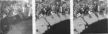
Figure 2: Band 3 of the tested Landsat- TM image (left), the classified images obtained by the conventional method (middle), and by the proposed method (right).
(light gray: vegetation area, black: water body, dark gray: waste land, white: bare soil)
A four-layer MLP model (the input layer, 2 hidden layers and the output layer) was used in this study. The network consists of 9 input nodes (3 linguistic properties x 3 bands), 4 output nodes (4 categories), and 10 nodes in each hidden layer. The parameter selection is as follows: hand a in eq. (5) are set to 0.01 and 0.9, SSE in eq. (4) is set to 0.003, fdemon in eqs. (12) & (14) is set to 0.8, b and r in eq. (16) are set to 5 and 1 respectively.
A simultation has been performed using MATLAB program running on Pentium pro 200 workstation (64 MB RAM). For a training set of 740 sample patterns, the conventional neural network method used 3 min. On 265 epochs while the proposed method used 8 min, on 3, 766 epochs. After training process, a test set of 3,388 sample patterns was used to evaluate the classification performance of the two methods. The results are shown in Table 1.
From the table, the proposed method seems to work a little better. Its overall correct classification is about 97.2%, against 96.0% for the conventional method. This situation is explained by a better attribution in the proposed fuzzy method case of water body, waste land and bare soil categories, whereas the conventional method make less errors than the proposed method in one case which is vegetation category. The classified images resulted from both methods are also provided in Figure 2.
6. Conclusion
A supervised classification algorithm for multispectral satellite images based on fuzzy logic and neural network has been described. The application of this algorithm to classification of Landsat-TM data has been proposed. The results showed an improvement in classification performance comparing to the conventional neural network algorithm.
References
Abstract: In this paper we present an algorithm based on fuzzy logic and neural network for supervised classification of multi-spectral satellite images. To deal with fuzzy information, gray level values of each multi-bath pixel are converted into three linguistic properties. This provides feature vectors in term of fuzzy membership values to the input of a neural network while the output vector is defined in term of membership value of each category. Experiments were carried out using Landsat-Tm data and the results are compared to those obtained by the conventional neural network classifier.
1. Introduction
The multi-layer perceptron (MLP) using the back-propagation (BP) algorithm is the convectional neural network model widely used in the supervised classification of multispectral satellite image data. By using training pixels, the network can be trained adaptively by updating its connection weights. The desired output is clamped to two state values: 1 to 0 (state 1 for 'belong to' and state 0 for 'not belong to' a category) (McCelland, 1986; Rangsanseri, 1998). But in real world, an input feature may possess a property with a certain degree of confidence or a pattern may belong to more than one category.
To deal with this fuzzy classification problem, an algorithm based on fuzzy logic and neural network was proposed. This algorithm is capable of handling input features (gray level values in each multi-band pixel), present in the three linguistic properties corresponding to each input feature, to the input of a neural network while assign output membership values of each category lying in the range [0,1] instead of 0 or 1 to the output vectors (desired output vector). This provides scope for increases its robustness in tackling imprecise input specification and allows modeling of fuzzy data which may belong to more than one category.
The MLP model and BP algorithm is described in the first section. In the following section the fuzzy sets, the pattern representation in linguistic form and the membership of output vector are described. Then we explain the fuzzy extension to BP algorithm. Finally, the experimental results using Landsat-TM data are given and compared to those obtained by the conventional neural network classifier.
2. MLP Model and BP Algorithm
The MLP model using the BP algorithm consists of sets of nodes arranged in multiple layers called input, output, and hidden layers. Only the nodes of two different consecutive layers are connected by weights, but there is no connection among the nodes in the same layer. For all nodes , except the input layers nodes, the total input of each node is the sum of weighted outputs of the nodes in the previous layer. Each node is activated with the input to the node and the activation function of the node. The input and output of the node I (except for the input layer) in a MLP model according to the BP algorithm (Pao, 1989) is :
The sum in eq. (1) is over all nodes j is the previous layer. The Sigmoid function (McCelland, 1986) given in eq. (3) is used to determine the output state.
f(Xi)=1/(1+exp(-Xi)) (3)
where Wij is the weight of the connection from node i to node j, bi the numerical value called bias, and f() the activation function.
The BP algorithm is designed to reduce an error between the actual output and the desired output of the network in a gradient descent manner. The summed squared error (SSE) is defined as:
Where p indexes the all training patterns and i indexes the output nodes of the network. Opi and tpi denote the actual output and the desired output of node i, respectively, when the input vector p is applied to the network.
A set of representative input and output patterns is selected to train the network. The connection weight Wij are adjusted when each pattern is presented. All the patterns are repeatedly presented to the network until the SSE function is minimized. Application of the gradient descent method (Bendiktsson, 1990) yields the following iterative weight update rule:
DWij(n+1)=h(diOi)+aDWij(n) (5)
where Wij is the weight of the connection from node i to j, h the learning factor, a the momentum factor, and di the node error. For output node i, di is then given by:
di =(ti-Oi)Oi(1-Oi) (6)
The node error at an arbitrary hidden node i is:
3. Fuzzy Logic
In conventional neural network classifier, an element r either 'belong to' or 'not belong to' a given category A is expressed as:
Using fuzzy logic, the element r belonging to the universe R, may be assigned a grade of membership with the membership function mA( r ) to a fuzzy set A is defined as:
A={(mA(r),r)}, rÎR, mA( r )Î [0,1]
3.1 Pattern representation in linguistic form
Each input feature Fj be expressed in terms of membership values to each of the three linguistic properties: low, medium, and high. Therefore an n-band-pattern
will be represented as a 3n-dimension
vector. We use the membership function (Pal, 1992) with range [0,1] and r ÎRn which is defined as eq. (9) to convert Fj to its three-dimensional form which is given by eq. (8).
where l is the radius of the p functuion, c the central point, and || . || the Euclidean norm.
Note that, the membership value decreases when its distance from the central point c(||r-c||) increase. It is maximum (p=1) when the pattern r lies at the central point c of a category (||r-c||=0).
Let Fjmax and Fjmin are the upper and lower bounds of the feature Fj in all L pattern points. Then the three linguistic property sets are defined as :
where fdenom is the parameter controlling the extent of overlapping. The overlapping structure of the p functions for the three linguistic properties is shown in Figure 1.
Figure 1: Overlapping structure of the p functions for the three linguistic properties.
3.2 Category membership of output vector
We use the Beta membership function to define the desired output of the network (this allows the desired output, lies in the interval [0,1], not clamped to only state 1 (belong to a category) or state 0 (not belong to a category).
The Beta membership function of the ith pattern to the kth category, with range [0,1] are defined as:
Where Zik: the weight distance from the ith input pattern
to the center of the Kth
categoryb and p: the denominational and the exponential fuzzy generators which control the amount of fuzziness.
Mk: the mean of the mean of the numerical input patterns for the kth category
Fij: the value of the jth component of the ith pattern point.
Note that when the distance is 0 the membership value is 1 (maximum) and when the distance is infinite the membership value is 0 (minimum).
4. Fuzzy Extension to BP Algorithm
The fuzzy extension to BP algorithm consists of two steps. The first step is the fuzzy logic step. The p membership function (eqs. (8)-(15) are used to convert gray level values of each multi-band pixel into the three linguistic properties: low, medium, and high to the input vector of the network (So that, when we use n-band image, we will have 3n input nodes) and the Beta membership function (eqs. (16)-(17)) are used to define the desired output of the network (this allows the desired output, lies in the interval [0,1] not clamped to only state 1 (belong to a category) or state 0 (not belong to a category)). In the second step, the BP learning algorithm (eqs. (1)-(7)) are used to train the network until eq. (4) is minimized and the network "leans" the input patterns.
5. Experiments Results
A Landsat-TM image, over the area of Chumporn city, Thailand, taken on 10th March 1998 was used. The data consists of three bands including band 3(0.63-0.69 mm), band 4 (0.76-0.90 mm) and bands 5 (1.55-1.75 mm). The image size is 256*256 pixels. The aim of the classification was to distinguish between the 4 categories: vegetation area, water body, waste land and bare soil. From study area, 4,128 sample patterns are pick up randomly. A subset of 740 patterns in this set are used as training set, and residual 3,388 patterns are used as test set.
| Category | Number of pixels | Conventional method | Proposed method | |
| Training | Test | Correct (%) | Correct (%) | |
| 1. Vegetation | 272 | 1,243 | 1,185 (95.3) | 1, 159 (93.2) |
| 2. Water body | 198 | 870 | 843 (96.9) | 855 (98.3) |
| 3. Waste land | 126 | 824 | 787 (95.5) | 818 (99.3) |
| 4. Bare soil | 144 | 451 | 434 (96.2) | 442 (98.0) |
| Total | 740 | 3,388 | 3,249 (96.0) | 3,274 (97.2) |
Figure 2: Band 3 of the tested Landsat- TM image (left), the classified images obtained by the conventional method (middle), and by the proposed method (right).
(light gray: vegetation area, black: water body, dark gray: waste land, white: bare soil)
A four-layer MLP model (the input layer, 2 hidden layers and the output layer) was used in this study. The network consists of 9 input nodes (3 linguistic properties x 3 bands), 4 output nodes (4 categories), and 10 nodes in each hidden layer. The parameter selection is as follows: hand a in eq. (5) are set to 0.01 and 0.9, SSE in eq. (4) is set to 0.003, fdemon in eqs. (12) & (14) is set to 0.8, b and r in eq. (16) are set to 5 and 1 respectively.
A simultation has been performed using MATLAB program running on Pentium pro 200 workstation (64 MB RAM). For a training set of 740 sample patterns, the conventional neural network method used 3 min. On 265 epochs while the proposed method used 8 min, on 3, 766 epochs. After training process, a test set of 3,388 sample patterns was used to evaluate the classification performance of the two methods. The results are shown in Table 1.
From the table, the proposed method seems to work a little better. Its overall correct classification is about 97.2%, against 96.0% for the conventional method. This situation is explained by a better attribution in the proposed fuzzy method case of water body, waste land and bare soil categories, whereas the conventional method make less errors than the proposed method in one case which is vegetation category. The classified images resulted from both methods are also provided in Figure 2.
6. Conclusion
A supervised classification algorithm for multispectral satellite images based on fuzzy logic and neural network has been described. The application of this algorithm to classification of Landsat-TM data has been proposed. The results showed an improvement in classification performance comparing to the conventional neural network algorithm.
References
- Bendiktsson, J.A., Swain, P.H., and Ersoy, O.K., 1990. Neural network approaches versus statistical methods on classification of multisource remote sensing data. IEEE Trans. Geosci. Remote Sensing, 28(4), pp.540-552.
- MvCelland, J.L. and Rumelhart, D.E, Eds., 1986. Parallel distribution Processing, Vol.1. MIT Press, Cambridge, MA.
- Pal, S.K. and Mitra, S., 1992. Multilayer perceptron, fuzzy sets, and classification. IEEE Trans. Neural Network, 3(5), pp.683-697.
- Pao, Y.H., 1989. Adaptive. Pattern recognition and Neural Network. Addison-Wesley Publishing Company, Inc.
- Rangssanseri, Y., Thitimajshima, P., and Promchareon, S., 1998. A study of neural network classification of JERS-1/OPS images. In: 19th Asian Conference on Remote Sensing, pp.12-1-12-6.