Effects of JPEG Compression on Accuracy of Image Classification

Effects of JPEG Compression on Accuracy of Image Classification

Kent W. K. Lam*,W. L. Lau**,Z. L. Li***
*Assistant Professor, ** Research Assistant,
*** Associate Professor
Department of Land Surveying and Geo-Informatics
The Hong Kong Polytechnic University
HungHom, Kowloon, Hong Kong (CHINA)
Tel: (852)-27665962 Fax: (852)-23302994
E-mail: lskent/97980389r/lszlli@polyu.edu.hk

Keywords: JPEG, Image Compression, Image Classification, Remote Sensing

Abstract
Image classification strategies based on the multi-spectral imagery from satellite-based remote sensing have been widely applied in the extraction and classification of land use patterns and land coverage. One of the important elements which will affect the results of classification is the image quality. Recently, due to the large compression ratio achieved by lossy image compression algorithms, such as JPEG, those image compression techniques have gained a lot of attention from the remote sensing discipline. However, as computer based image analysis tools are very sensitive to image quality, small changes in the image content may affect the analysis results. The results after image classification using the compressed multi-spectral images will also be affected due to the deterioration of image quality as a result of increased compression ratio.

This paper describes some experimental investigations into the effect of JPEG compression on the accuracy of image classification using multispectral SPOT image. MLC supervised classification strategy was used for classification with vary compression quality factors. As a result of the investigation, it was found that images with high classification accuracy can be compressed more without too much effects on the overall accuracy of the classification. It is possible to compress a satellite image using a q-factor value of 35 with less than 3% lost of the classification accuracy. However, more experiments need to be conducted using images from different scenes with different land use coverages to support the above remark.

Introduction
Remotely sensing imagery captured from satellites has become one of the most important sources of spatial data for Geographical Information Systems (GIS). Without going through sophisticated processing, most of these images can be used immediately as background images once they are geographically referenced. To extract more information such as digital terrain model (DTM), land use patterns and land coverage, and ground features from the images, sophisticated processes are required to perform the tasks. To extract DTM, a pair of satellite images with overlapping coverage but taken from different locations in space is required. To extract ground features accurately from a satellite image, high resolution satellite image together with the corresponding DTM are needed. For the extraction and classification of land use patterns and land coverage, multi-spectral satellite imagery is required. Image classification strategies based on the multi-spectral imagery from satellite-based remote sensing have been widely applied. These strategies could either be categorized as supervised which the a-prior training data are needed for the discipline-dependence results, or unsupervised which are self-trained for the statistical patterns from the images. One of the important elements which will affect the results of any of the above three processes is the image quality.

Recently, due to the large compression ratio achieved by lossy image compression algorithms, such as JPEG, those image compression techniques have gained a lot of attention from the remote sensing discipline. Most of these lossy compression techniques are mainly designed to exploit human vision system limitations. The image quality of the compressed image is definitely affected but it may not be visible or obvious when examines by human eyes. However, as computer based image analysis tools are very sensitive to image quality, small changes in the image content may affect the analysis results. The results after image classification using the compressed multi-spectral images will also be affected due to the deterioration of image quality as a result of increased compression ratio. The effects of image compression on DTM accuracy were studied by Lam K.W.K. et.al.(1999). It was found that a near linear fall-off in accuracy with decreasing q-factor values (reducing quality settings) from 95 up to the value of 30. Errors increase by 60% when q-factor value is 20. Algarni (1996) conducted an experiment using an unsupervised classification strategy, ISODATA, to study the effect of JPEG compression on the geometric and visual quality of the output of compression using three TM band from LANDSAT. He concluded that only 4.5% pixels in a compressed image were mis-classified but the result could be scene dependent. This paper is to discuss the experimental results conducted on the accuracy of classification using maximum likelihood classifier (MLC) supervised classification strategy using SPOT multispectral images with vary compression quality factors.

Compression Quality Setting in Jpeg
JPEG image compression standard was introduced and developed by the Joint Photographic Experts Group (JPEG) has been working under the auspices of three major international standards organizations - International Organization for Standardization (ISO), the International Telegraph and Telephone Consultative Committee (CCITT), and the International Electrotechical Commission (IEC) - for the purpose of development a standard for color image compression (Pennebake and Mitchell, 1993). This standard provides a guideline for the software developers to implement according to their own specifications. JPEG is "lossy" and is intended for compressing images with little or no obvious changes identifiable by humans. Due to this highly efficient and effective compression techniques, JPEG compression techniques and the JPEG formats have been widely accepted in the remote sensing discipline to optimize data storage and to reduce data transmission time. With the recent announcement by Space Imaging of Denver, Colo. of the successful launch of the world’s first commercial, high-resolution imaging satellite, the importance of image compression for the storage and transmission of remotely sensed images become even more important.

Review of the JPEG compression standard would not be reported in this paper. Comprehensive discussion of the standard can be found in the book written by Pennebaker and Mitchell (1993) and the white papers by Lane (1999). A brief overview can also be found in Lam K.W.K. et. al. (1999). However, it is worth to note that JPEG is more than an algorithm for compression images but also architecture for a set of image compression functions suitable for a wide range of applications involving image compression. A useful property of the architecture of JPEG is to allow adjusting compression parameters (quality factor) to increase the degree of lossiness. Hence, one can trade off file size against image quality. However, as JPEG standard does not specify how quality scales should be implemented, different software developers may use different scales to control the quality factor (q-factor). The scale between 0-100 is the widely accepted scale range but the scale range has nothing to do with percentage of information to be kept in an image.

Accuracy Indicators for image Classification
The confusion matrix, sometimes called the error matrix, is almost universally adopted as the standard error report in supervised classification. The matrix is a symmetrical array of numbers, which express the number of classified pixels in the assigned category relative to the actual category from ground truth data (Table 1). The columns present the numbers of ground truth data while the numbers of classified pixels are indicated in the rows. Based on the differential analysis of elements in the matrix, the omission error, commission error and overall accuracy of classification can be computed. The diagonal element indicates the numbers of classified pixels belonging to that category and a greater value equals more pixels being “correctly” classified. Computation of overall accuracy with the diagonal elements by the weighting of total training pixels yields a more reliable assessment for a result. For example, the overall accuracy is (89+69+45)/223 = 91.03%. To simplify the comparative analysis of the confusion matrix, only the overall accuracy was considered in this study.

Table 1. An example of the confusion matrix

Classified Data		Ground Truth Data			Row Total
		A	B	C	Row Total
	A	89	2	3	94
	B	7	69	1	77
	C	3	4	45	52
	Column total	99	75	49	223

The principle of the Kappa coefficient is to measure the difference between the agreement of the working process and the agreement of chance in the assigning pixel. As the classifier can randomly assign the pixel into the “correct” category by chance, a pixel can be assigned to the feature either by the actual classification or by chance. To measure the difference of actual or chance process, the Kappa coefficient (K) is defined as the following equation 1:
K=(P₀-P_e)/(1-P_e) (1)
Subject to the numbers of observed (P_o) and expected (P_e) pixels, the percentage of their difference is computed as the coefficient. The observed pixel is represented by the accurate classified pixel, which is coming from the normalized sum of diagonal elements (ii), as equation 2. The expected number is represented by the designated number of pixels in the “correct” classification such as the training data or data verified by reference data, which is computed from normalized value of the row (i) and column (j) total in the confusion matrix, as equation 3. Thus, the mathematical representation of Po and Pe are given by the following:

For the computational purpose, the equation of Kappa coefficient (K) is:

where t is the number of rows in the error matrix,
N is the total number of training data in the error matrix As the pixels are referred to the elements of the confusion matrix, the coefficient includes the errors of omission and commission. A higher value indicates that the result is in better classification than the random assignment. For example, K with value 0.86 is interpreted that a classified image achieves an accuracy that is 86 percent better than the chance assignment of pixels to categories. Hence, this coefficient implies the reliability of the classification agreement.

Test Areas
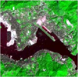
Experiments were conducted using sub-scenes from SPOT XS image taken on February 5, 1995 by SPOT-2 satellite with image resolution of 20m. Both sub-scenes were extracted from the image with image dimension 512x512 pixels. The first scene, Hong Kong CBD, covers the central business area which includes the Kowloon peninsula, the Victoria Harbour and the Northern district of the Hong Kong Island (Figure 1). The second scene, Tuen Mun, covers the Tuen Mun new town located in the North West Territories of Hong Kong (Figure 2).


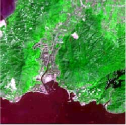Figure 1. Scene of Hong Kong CBD	Figure 2. Scene of Tuen Mun

Both scenes have similar ground coverages but with different land use patterns. The following three different ground coverages, urban area, vegetation and water, can easily been identified from the scenes. PCI image processing software running on a SUN Solaris UNIX platform was used to conduct the experiments. For image compression, the JPEG baseline compression software was used for image compression. For the supervised image classification strategy, the maximum likelihood classifier (MLC) was selected. Five classes: water (WATER), vegetation (VEG), mixed –urban (URBAN) and barren (BARREN) are defined as the extracted categories. Null class is allowed. All the results with different q-factors are then assessed and quantified by the overall accuracy and Kappa coefficient based on the confusion matrix. Without any compression, the overall accuracy for the scene, Hong Kong CBD, is about 93% but the overall accuracy for the scene, Tuen Mun, is only 85%.

Experimental Results and Analysis
Both sub-scenes of the SPOT image were compressed using the JPEG baseline compression algorithm provided by the PCI software. Starting from a q-factor of 100, the original images were compressed with a q-factor step size of 5 until the q-factor value reached 0 but q-factor 1 was used instead. Since both images have similar land use coverages and they were both extracted from the same SPOT image, the two curves illustrated by Figure 3 show that both images have also identical compression characteristics. The compression ratio reduces very rapidly as the q-factor value changes from 100 to 70. This result seems to agree with the q-factor value of 75 as suggested by the PCI software. However, Figure 3 only illustrates the relationship between q-factor and compression ratio but does not indicate the effects on the accuracy of the classification process.

Figure 3. Compression Ratio vs. Q-Factor for the Two Sub-scenes

Figure 4 below illustrates the relationship of the overall accuracy and the Kappa coefficient against the JPEG q-factor for both images. For the CBD image, by changing the q-factor value from 100 to 35, the accuracy of the classification as illustrates by both the overall accuracy and the Kappa coefficient can still be maintained in a very high level. The overall accuracy reduces from 93.19 (original without compression) to 92.01(q-factor value 35), and Kappa coefficient changes from 0.904(original without compression) to 0.888(q-factor 35). Only 3% of the classification accuracy is lost as compared to the original classification accuracy. For the Tuen Mun image, the overall accuracy reduces from 85.24 (original without compression) to 72.82 (q-factor 35), and Kappa coefficient changes from 0.804(original without compression) to 0.633(q-factor 35). A 15-20% accuracy reduction was experienced as compared to the classification accuracy using image without compression. The above results seem to suggest that there is a relationship between the compression ratio and the accuracy of the classification. Images with high classification accuracy can be compressed more without too much effect on the overall accuracy of the classification. Images with lower classification accuracy will suffer further from the image degradation effect as a result of using a lower JPEG q-factor.

Figure 4. Classification Accuracy vs. Q-Factor for the Two Sub-scenes

Conclusion
Hence, it is possible to compress a satellite image using a q-factor value of 35 with less than 3% lost of the classification accuracy. A q-factor value of 35 is able to achieve a compression ratio of 0.09, 9% of the size of the original image without compression. Of course, the above conclusion remark may not be accurate because only two images were used to conduct the experiment. In addition, only the MLC supervised classification strategy was selected to perform the supervised classification. Therefore, more experiments need to be conducted using images from different scenes with different land use coverages. Different types of supervised classification strategies should also be used to conduct the experiments.

Acknowledgements
The work described in this paper was substantially supported by a grant from the Research Grants Council of the Hong Kong Special Administrative Region (Project No. PolyU 5091/97E).

References

Algarni D.A., 1996. Compression of Remotely Sensed Data Using JPEG, International Archives of Photogrammetry and Remote Sensing. Vol. XXXI, Part B3, Vienna 1996, pp. 24-28.
Lane, T. (Maintainer), 1999. JPEG image compression FAQ, part 1 and part 2. http:///www.faqs.org/faqs/jpeg-faq/.
Lam, K.W.K. Nelson F. S. Chan and Zhilin Li, 1999. The Effects of Image Compression on DTM Accuracy, Proceedings of The International Symposium on Spatial Data Quality’99, pp. 228-235.
Pennebaker W. B. and J. L. Mitchell, 1993. JPEG Still Image Data Compression Standard, Van Nostrand Reinhold, New York.