| GISdevelopment.net ---> AARS ---> ACRS 1999 ---> Hyper Spectral Image Processing |
Spectral Mixture Analysis of
Hyperspectral Data
Yi-Hsing Tseng
Associate Professor, Department of Surveying Engineering
National Cheng Kung University
#1 University Road, Tainan, China Taipei
Tel: (886)-6-2757575-63835 Fax: (886)-6-2375764
Email: tseng@mail.ncku.edu.tw
Associate Professor, Department of Surveying Engineering
National Cheng Kung University
#1 University Road, Tainan, China Taipei
Tel: (886)-6-2757575-63835 Fax: (886)-6-2375764
Email: tseng@mail.ncku.edu.tw
Keywords: Spectral Mixture Analysis, Spectral
Unmixing, Hyperspectral Data þ
Abstract
Spectral mixture analysis of hyperspectral data is performed to validate the spectral unmixing technique worked based on the theory of linear mixture modeling. High-resolution spectra of mixed soil and vegetation were collected for the analysis using a field spectrometer. The instrument FOV was carefully validated to ensure the correctness the mixture proportions of the sensed materials. A data set of designed sample targets with linear variation of mixture proportions was collected. The data quality and the solution of single-band unmixing were then investigated in the spectral space. Based on the analysis, a weighted least-squares method is suggested to reinforce the solution of spectral unmixing.
1. Introduction
In remote-sensing imagery, the measured spectral radiance of a pixel is the integration of the radiance reflected from all the objects within the ground instantaneous field of view (GIFOV). Mixed pixels are generated if the size of the pixel includes more than one type of terrain cover. Obviously, spectral mixing is inherent in any finite-resolution digital imagery of a heterogeneous surface. Solving the spectral mixture problem (Horwitz et al., 1971) is, therefore, involved in image classification, referring to the technique of spectral unmixing. The application of spectral unmixing was limited due to the low spectral resolution of the sensors in the past. The invention of imaging spectrometers (Goetz et al., 1985) promotes the potential of applying spectral unmixing for image classification. The large number of spectral bands in hyperspectral data allows the unmixing of very complex scenes to avoid intrinsic singular problems. In addition, the hyperspectral data permits the direct identification of image-derived endmember spectra (Boardman, 1994). However, the spectral mixing behaviors are still not clearly known and modeled. Therefore, how muck these unknown behaviors will affect the solution of spectral unmixing should be studied carefully.
Conceptually, the occurrence of multiple materials, or endmembers, within the GIFOV of a single pixel leads to a composite or mixed spectral signal. The spectra of an endmember ideally represent the signatures that would be recorded for pure or single-component pixels. A pixel composed of multiple components can be mathematically approximated using a spectral mixing model. Linear mixture modeling is commonly applied with the assumptions that electromagnetic energy reflected from the surface interacts with a single component (Adams et al., 1986) and a uniform weighting of radiance over the GIFOV area. However, non-linear mixing may dominate frequently in reality when incident electromagnetic energy reacts with more than one component before being reflected from the surface, for example the reflectance from vegetation canopy. In addition, due to the fact that the sensor spatial spread function results in a non-uniform response, spectrally determinate fraction coefficients do not correspond with the proportions of endmembers distributed within a pixel. Certainly, the solution may be distorted if a non-linear mixture case is treated as a linear case or the sensor problem is ignored. Focused on the spectral mixing behaviors, this paper estimates the feasibility of the linear mixture modeling.
2. Spectral Unmixing Based on the Linear Mixture Model
With known number of endmembers and giving the spectra of each pure component, the observed pixel value in any spectral band is modeled by the linear combination of the spectral response of component within the pixel. This linear mixture model can be mathematically described as a linear vector-matrix equation,
where:
i = 1,. . .,m (number of bands);
j = 1,. . .,n (number of endmembers);
DNi = spectral reflectance of the ith spectral band of a pixel;
Rij = known spectral reflectance of the jth component;
Fj = the fraction coefficient of the jth component within the pixel;
Ei = error for the ith spectral band.
The error terms account for the unmodeled reflectance and represent the unknown noise of observations. The relationship in Eq. (1) is constrained by the assumption that an exhaustive set of endmembers (classes) has been defined, so that,
at each pixel. This assumption could be problematic, since one is never sure that a sufficient number of endmembers has been defined for a given set of data.
Using the constrained least squares (CLS) method proposed by Shimabukuro (1991) can solve the inversion problem, termed spectral unmixing. The objective of this method is to estimate the fraction coefficients by minimizing the sum of the squares of the errors, subject to the constraint given by Eq. (2). The estimated standard deviation of the error terms,
can be a quantitative measure of how the mixture modeling fits the data.
3. Data Collection and Fov Test
The GER 1500, a field portable spectroradiometer, is used for spectral data collection. This instrument is capable to read 512 spectral bands, covering the UV, Visible, and NIR wavelengths from 350 nm to 1050 nm. The instrument FOV is 4 degrees, and a sighting laser is provided to aid in aligning the instrument to the target to be measured.
Knowing the sensed area of the target surface covered by the instrument FOV with a certain shooting distance is important for the experiments of spectral mixture. Ideally, according to the calibrated FOV diagram provided with the instrument (GER, 1999), one can exactly know the area of sensed region (figure 1). However, we found that this data is not quite right. An experiment was, therefore, performed to test the real FOV. In this experiment, the sensor was set up to aim a black board with a shooting distance of 97 cm, and was kept stationary. The size of the black board is 20 by 20 cm, much larger than the expected FOV area. Then, a 1-cm wide white strip was moving 1 cm each time from left to right and from top to bottom over the black board, as sketched in figure 2. Spectral data were collected for each movement. The overlapped area of the white strip and the FOV area, therefore, can be estimated by calculating the spectral distance between each measurement and the background spectra. Figure 3(a) shows the spectral distances of the horizontal movement, and that of the vertical movement are shown in figure 3(b). Finally, the estimated FOV area and its center position relative to the laser spot are sketched in figure 4. The shape of the FOV area is obviously not a square. It could also be true that the GIFOV of most scanners is not a square either. It means that the fraction coefficients derived from spectral unmixing do not correspond with the proportions of the þ endmembers distributed within a square pixel. A variation of a spatial distribution of objects within a pixel would result in a large difference.
Figure 1: The FOV area of the GER 1500 with a shooting distance of 97 cm.
Figure 2: The FOV test experiment setup.
Figure 3: The spectral distance
between each measurement and the background spectra measured in the FOV
test
Figure 4: the estimated FOV area and its center position relative to the laser spot.
In addition, the boundary of the sensed region is not a clear cut, due to the sensor spatial spread function (Wu and Schowengerdt, 1993). This could be another factor that would distort a spectral mixture. To avoid this problem in data collection, the size of target objects should be smaller than the FOV area.
4. Test Data
A data set was collected to test how the spectral mixture modeling fits the real data. The target objects are two mixed materials, a soil region as the background and a proportionally increased vegetated area as the foreground. In order to ensure the proportion of the foreground is linearly increasing, 8 pie-shape green leaves in the same size were piece-by-piece put into the sensed region, as shown in figure 5. If the area of a green leaf is x% of the FOV area, the mixed proportions of the foreground will be 0%, x%, 2x%,…,8x%, and 100%. For each mixture, 10 sample data were collected. The spectral curves of all the sample data are shown in figure 6. The estimated spectral noises based on the collected data are shown in figure 7. The measures of spectral distance between each mixture and the pure background in feature space are also graphically shown in figure 8. The distance increases linearly with respect to the increase of foreground percentage.
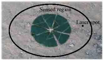
Figure 5: The distribution of the target objects for the data collection.
Figure 6: The spectral curves of the sample data.
Figure 7: Estimated spectral noises.
Figure 8: Spectral distance variation.
5. Spectral Unmixing Analysis
The spectral mixture of only two materials can be solved with the data of each band. According to Eq.(1), the ith spectral band is mixed as:
DNi=(Ri1*F1+Ri2*Ei (4)
Combining Eq.(4) with the constraint expressed in Eq.(2), one can solve F1 as following,
Let F1 be the fraction coefficient of the vegetation foreground, then the solutions of F1 in each band for all the sample data in the data set can be shown graphically in figure 9. Unstable solutions are obtained when the spectral band has almost the same reflectance, i.e., Ri1»Ri2. Removing the unstable solutions, the variation of the solutions can be clearly shown in figure 10. Linearity of spectral mixing can be validated in most of the bands except the absorption bands. One can remark that while most of the spectral bands provide positive effects, there are some spectral bands may contaminate the solution.
Figure 9: The solution of F1.
Figure 10: The solution of F1 after removing unstable ones.
For each sample data, the fraction coefficients were also calculated by using CLS. The results are graphically shown in figure 11. As mentioned above, the spectral bands do not have equal contributions to the solution of spectral unmixing. In addition, as shown in figure 7, the bands do not contain equal noise either. A weighted least squares (WLS) computation is, therefore, proposed to improve the solution. The discrepancy of band reflectance between endmembers and the noise level of measurements can be the reference to adjust the weights. The final results are graphically shown in figure 11.
Figure 11: CLS solutions.
Figure 12: WLS solutions.
Conclusding Remarks
A pixel-covered area is commonly recognized as a square. However, the shape of the GIFOV is actually not a square. This situation causes a problem that the fraction coefficients derived from spectral unmixing do not correspond with the proportions of the þ endmembers distributed within a square pixel. A variation of a spatial distribution of objects within a pixel would result in a large difference.
Due to the differences of the discrepancy of band reflectance between endmembers and the noise level of measurements, the spectral bands do not have equal contributions to the solution of spectral unmixing. A weighted least squares (WLS) computation is proved to be effective for improving the solution of spectral unmixing.
Acknowledgements
This research project was sponsored by the National Science Council of Republic of China under the grants of NSC88-2211-E006-051.
References
Abstract
Spectral mixture analysis of hyperspectral data is performed to validate the spectral unmixing technique worked based on the theory of linear mixture modeling. High-resolution spectra of mixed soil and vegetation were collected for the analysis using a field spectrometer. The instrument FOV was carefully validated to ensure the correctness the mixture proportions of the sensed materials. A data set of designed sample targets with linear variation of mixture proportions was collected. The data quality and the solution of single-band unmixing were then investigated in the spectral space. Based on the analysis, a weighted least-squares method is suggested to reinforce the solution of spectral unmixing.
1. Introduction
In remote-sensing imagery, the measured spectral radiance of a pixel is the integration of the radiance reflected from all the objects within the ground instantaneous field of view (GIFOV). Mixed pixels are generated if the size of the pixel includes more than one type of terrain cover. Obviously, spectral mixing is inherent in any finite-resolution digital imagery of a heterogeneous surface. Solving the spectral mixture problem (Horwitz et al., 1971) is, therefore, involved in image classification, referring to the technique of spectral unmixing. The application of spectral unmixing was limited due to the low spectral resolution of the sensors in the past. The invention of imaging spectrometers (Goetz et al., 1985) promotes the potential of applying spectral unmixing for image classification. The large number of spectral bands in hyperspectral data allows the unmixing of very complex scenes to avoid intrinsic singular problems. In addition, the hyperspectral data permits the direct identification of image-derived endmember spectra (Boardman, 1994). However, the spectral mixing behaviors are still not clearly known and modeled. Therefore, how muck these unknown behaviors will affect the solution of spectral unmixing should be studied carefully.
Conceptually, the occurrence of multiple materials, or endmembers, within the GIFOV of a single pixel leads to a composite or mixed spectral signal. The spectra of an endmember ideally represent the signatures that would be recorded for pure or single-component pixels. A pixel composed of multiple components can be mathematically approximated using a spectral mixing model. Linear mixture modeling is commonly applied with the assumptions that electromagnetic energy reflected from the surface interacts with a single component (Adams et al., 1986) and a uniform weighting of radiance over the GIFOV area. However, non-linear mixing may dominate frequently in reality when incident electromagnetic energy reacts with more than one component before being reflected from the surface, for example the reflectance from vegetation canopy. In addition, due to the fact that the sensor spatial spread function results in a non-uniform response, spectrally determinate fraction coefficients do not correspond with the proportions of endmembers distributed within a pixel. Certainly, the solution may be distorted if a non-linear mixture case is treated as a linear case or the sensor problem is ignored. Focused on the spectral mixing behaviors, this paper estimates the feasibility of the linear mixture modeling.
2. Spectral Unmixing Based on the Linear Mixture Model
With known number of endmembers and giving the spectra of each pure component, the observed pixel value in any spectral band is modeled by the linear combination of the spectral response of component within the pixel. This linear mixture model can be mathematically described as a linear vector-matrix equation,
where:
i = 1,. . .,m (number of bands);
j = 1,. . .,n (number of endmembers);
DNi = spectral reflectance of the ith spectral band of a pixel;
Rij = known spectral reflectance of the jth component;
Fj = the fraction coefficient of the jth component within the pixel;
Ei = error for the ith spectral band.
The error terms account for the unmodeled reflectance and represent the unknown noise of observations. The relationship in Eq. (1) is constrained by the assumption that an exhaustive set of endmembers (classes) has been defined, so that,
at each pixel. This assumption could be problematic, since one is never sure that a sufficient number of endmembers has been defined for a given set of data.
Using the constrained least squares (CLS) method proposed by Shimabukuro (1991) can solve the inversion problem, termed spectral unmixing. The objective of this method is to estimate the fraction coefficients by minimizing the sum of the squares of the errors, subject to the constraint given by Eq. (2). The estimated standard deviation of the error terms,
can be a quantitative measure of how the mixture modeling fits the data.
3. Data Collection and Fov Test
The GER 1500, a field portable spectroradiometer, is used for spectral data collection. This instrument is capable to read 512 spectral bands, covering the UV, Visible, and NIR wavelengths from 350 nm to 1050 nm. The instrument FOV is 4 degrees, and a sighting laser is provided to aid in aligning the instrument to the target to be measured.
Knowing the sensed area of the target surface covered by the instrument FOV with a certain shooting distance is important for the experiments of spectral mixture. Ideally, according to the calibrated FOV diagram provided with the instrument (GER, 1999), one can exactly know the area of sensed region (figure 1). However, we found that this data is not quite right. An experiment was, therefore, performed to test the real FOV. In this experiment, the sensor was set up to aim a black board with a shooting distance of 97 cm, and was kept stationary. The size of the black board is 20 by 20 cm, much larger than the expected FOV area. Then, a 1-cm wide white strip was moving 1 cm each time from left to right and from top to bottom over the black board, as sketched in figure 2. Spectral data were collected for each movement. The overlapped area of the white strip and the FOV area, therefore, can be estimated by calculating the spectral distance between each measurement and the background spectra. Figure 3(a) shows the spectral distances of the horizontal movement, and that of the vertical movement are shown in figure 3(b). Finally, the estimated FOV area and its center position relative to the laser spot are sketched in figure 4. The shape of the FOV area is obviously not a square. It could also be true that the GIFOV of most scanners is not a square either. It means that the fraction coefficients derived from spectral unmixing do not correspond with the proportions of the þ endmembers distributed within a square pixel. A variation of a spatial distribution of objects within a pixel would result in a large difference.
Figure 1: The FOV area of the GER 1500 with a shooting distance of 97 cm.
Figure 2: The FOV test experiment setup.
 (a) the horizontal movement |
 (b) the vertical movement |
Figure 4: the estimated FOV area and its center position relative to the laser spot.
In addition, the boundary of the sensed region is not a clear cut, due to the sensor spatial spread function (Wu and Schowengerdt, 1993). This could be another factor that would distort a spectral mixture. To avoid this problem in data collection, the size of target objects should be smaller than the FOV area.
4. Test Data
A data set was collected to test how the spectral mixture modeling fits the real data. The target objects are two mixed materials, a soil region as the background and a proportionally increased vegetated area as the foreground. In order to ensure the proportion of the foreground is linearly increasing, 8 pie-shape green leaves in the same size were piece-by-piece put into the sensed region, as shown in figure 5. If the area of a green leaf is x% of the FOV area, the mixed proportions of the foreground will be 0%, x%, 2x%,…,8x%, and 100%. For each mixture, 10 sample data were collected. The spectral curves of all the sample data are shown in figure 6. The estimated spectral noises based on the collected data are shown in figure 7. The measures of spectral distance between each mixture and the pure background in feature space are also graphically shown in figure 8. The distance increases linearly with respect to the increase of foreground percentage.
Figure 5: The distribution of the target objects for the data collection.
Figure 6: The spectral curves of the sample data.
Figure 7: Estimated spectral noises.
Figure 8: Spectral distance variation.
5. Spectral Unmixing Analysis
The spectral mixture of only two materials can be solved with the data of each band. According to Eq.(1), the ith spectral band is mixed as:
Combining Eq.(4) with the constraint expressed in Eq.(2), one can solve F1 as following,
Let F1 be the fraction coefficient of the vegetation foreground, then the solutions of F1 in each band for all the sample data in the data set can be shown graphically in figure 9. Unstable solutions are obtained when the spectral band has almost the same reflectance, i.e., Ri1»Ri2. Removing the unstable solutions, the variation of the solutions can be clearly shown in figure 10. Linearity of spectral mixing can be validated in most of the bands except the absorption bands. One can remark that while most of the spectral bands provide positive effects, there are some spectral bands may contaminate the solution.
Figure 9: The solution of F1.
Figure 10: The solution of F1 after removing unstable ones.
For each sample data, the fraction coefficients were also calculated by using CLS. The results are graphically shown in figure 11. As mentioned above, the spectral bands do not have equal contributions to the solution of spectral unmixing. In addition, as shown in figure 7, the bands do not contain equal noise either. A weighted least squares (WLS) computation is, therefore, proposed to improve the solution. The discrepancy of band reflectance between endmembers and the noise level of measurements can be the reference to adjust the weights. The final results are graphically shown in figure 11.
Figure 11: CLS solutions.
Figure 12: WLS solutions.
Conclusding Remarks
A pixel-covered area is commonly recognized as a square. However, the shape of the GIFOV is actually not a square. This situation causes a problem that the fraction coefficients derived from spectral unmixing do not correspond with the proportions of the þ endmembers distributed within a square pixel. A variation of a spatial distribution of objects within a pixel would result in a large difference.
Due to the differences of the discrepancy of band reflectance between endmembers and the noise level of measurements, the spectral bands do not have equal contributions to the solution of spectral unmixing. A weighted least squares (WLS) computation is proved to be effective for improving the solution of spectral unmixing.
Acknowledgements
This research project was sponsored by the National Science Council of Republic of China under the grants of NSC88-2211-E006-051.
References
- Adams, J.B., M.O. Smith, and P.E. Johnson, 1986. Spectral mixture modeling: A new analysis of rock and soil types at the Viking Lander 1 site. Journal of Geophysical Research, vol. 91(B8), pp. 8090-8112.
- Boardman, J.W., 1994. Geometric mixture analysis of imaging spectrometry data. In: Geoscience and Remote Sensing Symposium, IGARSS ’94, Surface and atmospheric remote sensing: technologies, data analysis and interpretation, vol. 4, pp. 2369-2371.
- Goetz, A.F.H., G. Vane, J.E. Solomon and B.N. Rock, 1985. Imaging spectrometry for Earth remote sensing. Science, vol. 228, pp. 1147-1153.
- Geophysical & Environmental Research Corp., 1999. GER 1500 Spectroradiometer user manual, Release 2.4.
- Horwitz, H.M., R.F. Nalepka, P.D. Hyde and J.P. Morgenstern, 1971. Estimating the proportions of objects within a single resolution element of a multispectral scanner. In: Proceedings of the 7 th International Symposium on Remote Sensing of Environment, Ann Arbor, Michigan, pp. 1307-1320.
- Shimabukuro, Y.E. and J.A. Smith, 1991. The least-squares mixing models to generate fraction images derived from remote sensing multispectral data. IEEE Transaction on Geoscience and Remote Sensing, vol. 29(1), pp. 16-20.
- Wu, H.-H.P. and R.A. Schowengerdt, 1993. Improved fraction image estimation using image restoration. IEEE Transaction on Geoscience and Remote Sensing, vol.31(4), pp. 771-778.