| GISdevelopment.net ---> AARS ---> ACRS 1999 ---> Hyper Spectral Image Processing |
A New Approach on Operational
Offshore Suspended Sediment Algorithm for Satellite Images
Ming Deng1, Yan
Li1, Jujie Yang2, Jin Li2, Shujing
Li1
1 the Second Institute of Oceanography, Hangzhou, 310012
2 Peking University, Beijing, 100871
Key words: remote sensing, suspended
sediment concentration, slope algorithm. 1 the Second Institute of Oceanography, Hangzhou, 310012
2 Peking University, Beijing, 100871
Abstract
Remote sensing in detecting offshore-suspended sediment is one of the important tasks of ocean research. Currently most achievements in this field focus on the low SSC (Suspended Sediment Concentration). However, in China the offshore environment is characterized turbid water with high SSC. This background makes the research in high SSC becomes a special and urgent task of China.
In marine remote sensing, how to remove atmosphere effect is a crucial and necessary step because only about 30% of the single detected by sensors is valid (Hovis and Leung, 1997). And the most difficult point is high SSC remote sensing is it too. Recently a new method, slope algorithm, is put forward by LiYan and Lijin (1998, 1999) to solve this problem. To put it into operational system and test this algorithm, we select the coast of East China Sea, including Chandjiang Estuary and Hangzhou Bay which are famous for their high SSC, as our study area, NOAA14/AVHRR CH1 and CH2 as data source and realize this algorithm through computer program. Preliminary long time series of SSC images have been acquired successfully. In this paper we will illustrate the following aspects in detail: general construction, solution to the difficult and key points, discussion about its feasibility, stability and application.
1 Fundamental about the slope algorithm
The water-leaving reflectance of sea surface changes greatly in the transmitting process. If consider two different bands, it can be proved that the change in the slope of their relation curve is linear in the transmitting process, namely the relation curve of water-leaving reflectance is similar with that of the reflectance detected by remote sensor. It is just through the relation between slopes, atmospheric effects, including high SSC areas, can be corrected. And the next, through the relation between water-leaving reflectance of sea surface and SSC to deduce the relation between slope and SSC, thus SSC can be calculated out (Li Yan, Li Jin, 1998; 1999).
2 Basis for programming algorithm design
The key step in carrying out this algorithm on computer is how to get the relationship curve of CH1/CH2 and corresponding slope from NOAA/AVHRR CH1 and CH2 images.
The following basic facts are the basis for the computer algorithm design:
- Relation between CH1 and CH2: (see fig.1) the two have the same alteration trends. For example, when CH1 increase, CH2 increases too. And it is clear that the relation curve can be simulated with linear equation or quadratic equation.
- Relation among CH1, CH2, K (Slope) and SSC: (see if.1) simply say, Ch1 µ K µ SSC and CH2 µ K µ SSC.
- Sensitivity of CH1 and CH2 to SSC: (see fig. 1). For low SSC, CH1 is more sensitive than CH2; and for high SSC, to the contrary. This phenomenon is related with the fact that as SSC increases its peak value of reflectance moves to the long wave (Chen Tao et al. , 1994).
- Special 'inversion': When SSC is very high, CH1 stop increasing and even decrease while Ch2 can maintain increasing to some degree, which makes the relation curve of CH1 and CH2 appears to reverse (see fig.2). It often happens at the shoals covered with very shallow water.
- Asymmetry of atmosphere: the general relationship between CH1 and CH2 has been stated in fact 1. but notice that because of the asymmetry of atmosphere, its concrete form is fluctuant at different places and in different times (see fig.2).
- Influence of cloud over sea: sometimes it is too difficult to distinguish them from water, especially the thin cloud or fog, which often lead to wrong results.
In practice, we take two methods, simulation method and max method.
Fig.1 CH1_CH2 relation curve (1997/10/16)
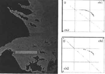
Fig. 2 the influence of atmospheric asymmetry.
3. Simulation
3.1 Basic steps of program
This method directly uses spatial local area and gray level local area to acquire slope K.
The basic steps are;
- Constructing a rectangle block (spatial local area) around current pixel (center point).
- Filtering initial gray data then get valid data through the predefined gray level local area.
- Using valid data to simulate the relation curve of CH1_CH2 (according to fact 1).
- Acquiring slope K and then SSC of current pixel from the simulation equation.
- Moving block one pixel by one until every pixel of image has been done with these steps.
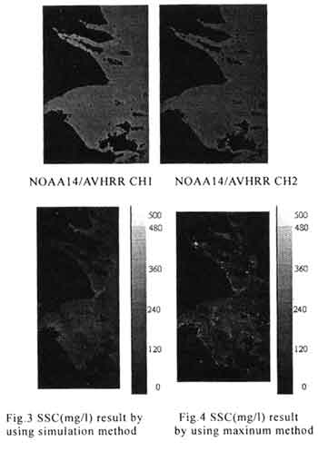
See fig.3. It is the SSC result image on 16th, Oct., 1997.
Our results show that the stability of slope is under the control of both spatial local area and gray level local area. To spatial local area, the smaller the block is, the better the result is. Because in small block the state of atmosphere could be considered as symmetry, which better ensures the accuracy of slope. But to gray level local area, the larger the block, the better. Because to simulate curve need enough statistic data. The conflict between the two local areas is the key and difficult point of the simulation method.
Presently, the following measures are taken:
- Changing the size of spatial local area according to the state of gray level local area in the block: to those having enough valid data in current gray level local area, keep the block size. To those having few valid data, enlarge the block size. In this way, not only get enough statistic data to simulate curve but also reduce the computing time.
- Changing range of gray level local area according to fact 3: to the clear water, relax the valid range of CH1 and reduce relax of CH2. To the turbid water, to the country.
- Independent variable alteration according to fact 3: choose CH1 as independent variable in the low SSC and choose CH2 in the high SSC.
4 Maximum method
4.1 Basic steps of program
Maximum method (LiYan, Lijing, 1998; 1999 ) is an in directed method to get slope.
It can be simply proved:
The slope (K) of CH1~CH2 relation curve can be expressed as:
K=dCH2/dCH1
Namely
K-dCH2/dCH1=0
Because K is a constant, there has:
d(K*CH1-CH2)/dCH1=0
This equation is just the discriminate function of the K*CH1-CH2 extremum. It can also prove this extremum is a maximum. Thus to get slope K could convert to get the max of K*CH1-CH2. Namely the distribution of K is equivalent to that of the max of K*CH1-CH2.
What we do in the practice is similar to that in the simulation method only different at the way we get slope. In every block, through calculating the max of K*CH1-CH2 to build the relation among K~CH1, CH2. Here K is preset (e.g., K= 0.02, 0.04 …….5 a arismetic series with step of 0.02).
4.2 Example and discussion
See fig.4. It is the SSC result image using maximum method on 16th , Oct., 1997.
Through the comparison of a number of result images, we find that:
- the conflict between spatial and gray level local area decrease: in the small block, K~CH1, CH2 strictly conform to fact 1,2 and does not appear fluctuation. While in bigger block, K~CH1, CH2 tend to be unstable and the bigger the block is the stronger this tendency is. It can be explained by that in big block the asymmetry of atmosphere get notable and influence the relation between.
- Limitation: the control of high side (e.g., in the above series refer to when K near to 5). It can be deemed that every gray point (determined by [CH1, CH2]) in block is a control condition of K~CH1, CH2. when K is at low side (e.g., when K = 0.02, then 0.04 ……). Because of many control point above it (e.g., when K= 0.02 then 0.04, 0.06 … 5 are all control point above it) , a gray point will not increase without limit. But when K is near to high side, control point decrease, and the last gray point are difficult to find its correct slope.
- It can't find its slope directly. For example, the center point is [68,56], and we only find 0.02~ [66,54], 0.08~ [73,62] directly. At this time we had to use the point we know to deduce the slope of center point.
- In maximum method, the influence of clouds is obvious.
- Getting rid of the highest point: namely delete the last section in the series of K~CH1, CH2 . Because of no control point above it, we consider that the last one is uncertain.
- Simple trend plane interpretation according to fact 2: for those that have not directly get slope. The result is related to the series of K~ CH1, CH2 and from this view max method still influenced by the conflict between spatial and gray level local area.
5. Error Comparison
A resulting the Changjiang Estuary shows that the maximum method is better than simulation method (See Fig.5). and we can see that to high SSC, the error of simulation method is apparent mainly caused by the fact 4 that we have stated before. And it means that the difference of two methods will enlarge within certain area.
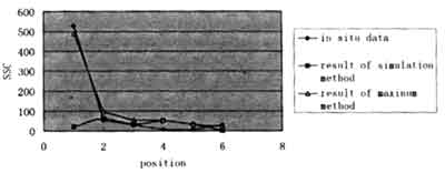
Fig 5. Comparison of calculating data with true data
6. Conclusion
Close to one hundred NOAA14/AVHRR CH1 and CH2 images, receiving 1997 and 1998, have been dealt with the Simulation Method and Maximum Method for the Slope algorithm. Compared with our accumulated historical data of the past experience (notice that it is difficult to get synchronous in situ data) most results are satisfying. Of course this new algorithm need much more in situ data to firmly confirm it.
We also notice the following problems: how to decrease the influence effectively when thin clouds or fog cover most of the research area; how to increase the sensitivity tot the very high SSC water.
References:
- Li Yan, Lijin, 1998, Maximum aR1-R2, the point for removal atmospheric effects from satellite imagery of the coast ocean, Proceeding of PORSC'98- Qingdao, Vol. 586-590.
- Li Yan and Li Jin, 1999, A suspended sediment Satellite sensing Algorithm based on Gradient Transiting from water-leaving to Satellite detected Reflectance Spectrum, Chinese Science Bulletin (Vol. 44, in press)
- Chen Tao , Li Wu, Wu Shuchu, The Relation between Suspended Sediment Concentration and the Peak Value of Light Spectrum Reflectance, ACTA OCEANOLOGICA SINICA, 1994 (Vol. 16, No. 1: 38-43)(Chinese edition).