| GISdevelopment.net ---> AARS ---> ACRS 1999 ---> GIS |
An Artificial Intelligent
Geographical-Spatial Model for Urban Transportation Travel Forecast
André Dantas and Yaeko
Yamashita and Eizo Hideshima and Koshi Yamamoto and Marcus V. Lamar
Nagoya Institute of Technology
Gokiso, Showa, Nagoya, 466-8555, Japan
Tel: (81) –52 – 735- 54 96 Fax: (81) –52 – 735- 54 96
E-Mail:andre@keik1.ace.nitech.ac.jp
Nagoya Institute of Technology
Gokiso, Showa, Nagoya, 466-8555, Japan
Tel: (81) –52 – 735- 54 96 Fax: (81) –52 – 735- 54 96
E-Mail:andre@keik1.ace.nitech.ac.jp
Keywords: Neural Networks, Remote Sensing, GIS,
Urban Transportation
Abstract
It is described in this paper a formulation of a travel forecast model that incorporates the geographical– spatial reality of urban areas. Throughout such incorporation, the model aims to characterize the interaction between land use – transportation system, which is the basis to represent the displacements (trips) needs of human activities within the urban area. Geographical Information System, Remote Sensing are explored in the obtainment and processing of geographical– spatial data, mainly originated from satellite and aerial photograph images. The comprehension of urban dynamics that affect travel process is established through an “artificial intelligent” approach using Neural Networks. A case study is conducted in order to evaluate and discuss NN modelling for travel forecast.
1. Introduction
In order to analyze urban area problems, Remote Sensing (RS) and Geographical Information Systems (GIS) integration has been successfully applied. Morain and Baros (1996) verified that RS-GIS integration data has lead to time reduction and cost-saving benefits against field surveys that are hardly updated by using traditional methods. However, Foresman and Millete (1997) emphasize that GIS capabilities have been concentrated in boolean operations and conventional spatial statistics when processing multilayered map-based information that has lead to a basic level of “display analysis”.
Recently, many efforts are observed intending to achieve more powerful spatial analytic and spatial process modelling tools by exploring Neural Networks (NN). According to Fischer (1999), computational geographers have faced NN as an instrument to overcome limitations of conventional tools to explore patterns and relationships in GIS and RS. Openshaw (1991) and Openshaw et al (1995) reported successful applications and NN efficiency, showing perspectives to elaborate a new modelling style. In this sense, it is essential to create models concerning this potential when integrated to GIS and RS.
Such potential is decisive to provide an efficient representation of urban dynamic that directly affects problems and solutions into the city. Specifically in transportation studies, travel demand is a consequence of how urban activities are processed and organized. This process is represented by urban dynamic along the years. Traditional forecast models quantify how urban activities are converted into travels considering socioeconomic data (population, income, etc.). Differing from previous formulations, this research proposes that travel forecast can be achieved analyzing land use and transportation system interactions in a spatial-temporal evaluation. These interactions could not be an easy task using traditional mathematical and statistical tools, but the integration of RS, GIS and NN concentrates together elements that are capable to represent the spatial characteristics of this problem. RS and GIS contribute to provide land use and transportation system data/information, which are mainly collected from satellite images and aerial photographs. On the other hand, NN gives support to the complex analysis of the interactions along the time and space.
This paper emphasizes this integration and presents a preliminary formulation of travel forecast model considering only the spatial dimension. Mainly, it is aimed to define basic characteristics and NN structures that after will be part of the spatial-temporal model. These definitions play a decisive role, since model’s essence will be established from these activities. Tests for Boston Metropolitan Area were conducted in order to verify the efficiency using this type of networks.
2. RS and GIS and NN Integration Approach
This integration approach allows incorporating to travel forecast model spatial-temporal characteristics related to urban area activities. It is necessary to develop a framework that combines RS and GIS and NN potential, involving steps from the data collection until the visualization and result analysis. In the development process, it is important to be concerned about the capabilities of each integration element. In this section, the proposed integration was created considering the whole process and specially NN definition for modelling in spatial dimension. Then, it is focused on the process description emphasizing on the framework formation in order to evaluate future development needs. Specific issues related to format, resolution and sources integration are not treated here.
Five modules compose the integration, that are: RS data; Trips data; Maps data; GIS; and NN. In figure 1, it can be verified that the process starts with data obtainment that is associated to the correspondent module. Thus, satellite images and aerial photographs are stored in RS data Module (1). The origin / destination tables are organized in Trips data Module (2) and finally maps containing transportation system information (road, subway, train, bus, etc) are transferred to Maps data Module (3). The data from Module 1 suffers a preliminary treatment inside GIS Module (4), in order to process multispectral analysis and aerial photograph interpretation. From this treatment, land use patterns are reached and gather together with data from Module 2 and 3 inside GIS database. Spatial-temporal queries are processed using this database and the results are conducted to NN Module (5). In this module, query results are pre-processed and then divided in training and test data sets. NN software performs the training process defining a function that is tested and revised until reach the expected level of forecast. Finally, Module 5 returns to Module 4 (GIS), where travel forecast function is applied to a future scenario and then visualized and analyzed.
3. Neural Network Definition for Modelling in Spatial Dimension
As part of travel forecast model definition, spatial and temporal dimensions are separately analyzed. Spatial dimension is devoted to represent the basic relations between land use patterns and transportation system affecting travel demand in a static stage of time. In the sequence, it is described NN formulation for spatial dimension.
Consider an urban area, which is divided in Traffic Zones (TZ). Trips (Tij) between TZ pairs are verified, where i and j denote the origin and destination, respectively. Land use is expressed by occupied area of each pattern in each TZ, which is assigned to RLUTZ (Residential Land use) CLUTZ (Commercial Land use) SLUTZ (Service Land use). Transportation system is characterized by the extension of each mode in each zone, which is associated to RTSTZ (Road Transportation System), BTSTZ (Bus Transportation System), STSTZ (Subway Transportation System) and TTSTZ (Train Transportation System).
Figure 1: RS and GIS and NN integration for Travel Forecast Problem
To be processed as a feedforward Multilayer Perceptron (see Wasserman, 1989), these characteristics are transformed in input (X) and output (Y) vectors. Then, it is defined that X = (RLUi, CLUi, SLUi, RTSi, BTSi, STSi, TTSi, RLUj, CLUj, SLUj, RTSj, BTSj, STSj, TTSj) and Y= (Tij). Physically, it means that trips between two zones (i and j) are expressed in NN by the Land use and transportation systems indicators for each zone (origin and destination). As a typical NN, input, hidden and output layers compose it. Hidden layers (H) are composed by are hidden neuron units H1, H2, ... Hm connect input and output, expressed by X and Y, respectively, as shown by Figure 2.
Figure 2: Typical NN structure
The output of the neurons are calculated by:
where fa and fb are activation functions that are suggested, in this work, to be logistic bipolar and identity function, respectively. W and V weight matrixes are obtained by applying a backpropagation based training algorithm (Wasserman, 1989).
4. Preliminary Tests
Tests were conducted in Boston Metropolitan Area (Massachusetts State – USA) (see Figure 3a), which covers about 1400 square miles (3580 square kilometers) where nearly three million people live. It was selected a study area in Boston South area, near to Boston Medical Center that involves seventeen TZ`s as shown in Figure 3b. Study area is mainly occupied by residential land use and it is located very close to downtown.
RS and transportation system data were obtained from MassGIS database. In this database, data was projected to Massachusetts State plane Mainland Zone coordinate system, Datum NAD83 in meters. It was used black and white digital orthophotos produced in 1992 in 1:5000 scale. Bus route maps from Metropolitan Boston Transportation Authority (MBTA) were incorporated to Transportation data. Finally, Central Transportation Planning Staff (CTPS) provided access to travel data related to 1990 survey that involves all purposes trips as well as TZ definition.
In the sequence, GIS database construction activities are described and results of the experiments are introduced.
4.1 GIS database
Geoconcept GIS software was used in these tests. First, land use patterns were obtained following United States Geological Service (USGS) classification system (Avery and Berlin, 1990) and Taco’s methodology (Taco et al, 1999). It was analyzed up to Level II (Residential, Commercial and Services) according to model’s requirements (see item 3). Figure 3c presents the land use patterns for the study area. Next, transportation system was digitalized in the GIS database. Figure 3d shows road, bus, subway and train systems for study area.
4.2 NN experiments and results
After GIS database construction and spatial query processing, it was created a data set to be used in the experiments. Data were normalized using equation 3.
where xkTZ is the value from X vector for characteristic k (land use or transportation system) in traffic zone TZ and xnkTZ is the normalized value. xkmin and xkmax are the minimum and maximum values for the kth feature.
Using this normalized data set, five NN structures were simulated in T-learn NN software. From the basic structure described in item 3, it was established variations in hidden layer. Structures A, B and C were defined with 14, 28 and 7 units in hidden layer, respectively. In structure D and E, it was inserted one and two hidden layers, respectively. It was observed for all structures that after 100,000 sweeps that the networks get into the over-training (excess of training) state. Then, the more NN is trained, the more it will be restricted to express just the training data set, losing its generalization power. In this sense, the training is stooped when the minimum error for test data that is found using equation 4.
where MSE is the mean square error considering forecasted (Y) and expected (T) trips for p testing data vectors.
Figure 3a: Boston Metropolitan Area Source: MIT Digital orthophoto project http://ortho.mit.edu/
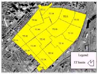
Figure 3b: Study area – selected Traffic Zones Figure 3d: Transportation System
Figure 3c: Land use patterns
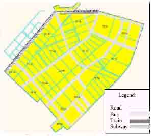
Figure 3d: Transportation System
It was verified that structure C presented the best result (MSE= 10) and structure A generated the worst MSE value (MSE= 11,21). This error variation range is quite narrow indicating that the network structure is not a fundamental parameter to obtain a good modelling.
Graph 1 shows expected (T) and forecasted (Y) trips generated by NN using the structure C as well the absolute difference between them. It can be observed how NN was able to model the relationship between input and output vectors in order to achieve a minimum error for travel forecast. The average error was 2.38 trips, which denotes a good result considering the complete data set. However, this error is high in some special cases where the network was not efficient to do the modelling, generating a considerable level of error. In these cases (vectors 32, 29, 7, 16, 16, 51 and 43), one or more characteristics of the input vector (X) were zero. It was generated due to the adoption of the Traffic Zone aggregation level that provided data for a very limited area, where some input vector characteristics do not exist. It is expected that NN can achieve a better level of forecast, if more aggregated areas are used. Additional tests are necessary to evaluate deeply these results in order to simulate some variations that could affect NN modeling. For instance, it is essential to analyze if the observed behavior for this study area is extended to the rest of Boston Metropolitan Area, which presents a large variety of urban activities and occupation.
5. Conclusions
It was described the development of a model to be applied in travel forecast activities under an “artificial intelligent” approach based on RS and GIS support. This approach intends to explore geographical-spatial-temporal data to express human being displacements needs in urban areas. It was discussed an integration framework that combines dynamically RS-GIS-NN to create information about travel process that is supposed to be used in transportation planning activities. Preliminary tests showed that selected characteristics are suitable to represent such problem. The results indicated that the established NN was capable to process the travel forecast modelling. It was also discussed the necessity to develop or select an aggregation level that can improve model’s efficiency. These improvements will be incorporated to the spatial-temporal model that is expected to forecast considering a multi-year evolution of land use patterns and transportation system.
Acknowledgments
The first author would like to express gratitude by the scholarship supported from Japanese Ministry of Education (Monbushou) for the development of this research. We also would like to thank Central Transportation Planning Staff (CTPS) of Boston for all support and travel data used in this research.
References
Abstract
It is described in this paper a formulation of a travel forecast model that incorporates the geographical– spatial reality of urban areas. Throughout such incorporation, the model aims to characterize the interaction between land use – transportation system, which is the basis to represent the displacements (trips) needs of human activities within the urban area. Geographical Information System, Remote Sensing are explored in the obtainment and processing of geographical– spatial data, mainly originated from satellite and aerial photograph images. The comprehension of urban dynamics that affect travel process is established through an “artificial intelligent” approach using Neural Networks. A case study is conducted in order to evaluate and discuss NN modelling for travel forecast.
1. Introduction
In order to analyze urban area problems, Remote Sensing (RS) and Geographical Information Systems (GIS) integration has been successfully applied. Morain and Baros (1996) verified that RS-GIS integration data has lead to time reduction and cost-saving benefits against field surveys that are hardly updated by using traditional methods. However, Foresman and Millete (1997) emphasize that GIS capabilities have been concentrated in boolean operations and conventional spatial statistics when processing multilayered map-based information that has lead to a basic level of “display analysis”.
Recently, many efforts are observed intending to achieve more powerful spatial analytic and spatial process modelling tools by exploring Neural Networks (NN). According to Fischer (1999), computational geographers have faced NN as an instrument to overcome limitations of conventional tools to explore patterns and relationships in GIS and RS. Openshaw (1991) and Openshaw et al (1995) reported successful applications and NN efficiency, showing perspectives to elaborate a new modelling style. In this sense, it is essential to create models concerning this potential when integrated to GIS and RS.
Such potential is decisive to provide an efficient representation of urban dynamic that directly affects problems and solutions into the city. Specifically in transportation studies, travel demand is a consequence of how urban activities are processed and organized. This process is represented by urban dynamic along the years. Traditional forecast models quantify how urban activities are converted into travels considering socioeconomic data (population, income, etc.). Differing from previous formulations, this research proposes that travel forecast can be achieved analyzing land use and transportation system interactions in a spatial-temporal evaluation. These interactions could not be an easy task using traditional mathematical and statistical tools, but the integration of RS, GIS and NN concentrates together elements that are capable to represent the spatial characteristics of this problem. RS and GIS contribute to provide land use and transportation system data/information, which are mainly collected from satellite images and aerial photographs. On the other hand, NN gives support to the complex analysis of the interactions along the time and space.
This paper emphasizes this integration and presents a preliminary formulation of travel forecast model considering only the spatial dimension. Mainly, it is aimed to define basic characteristics and NN structures that after will be part of the spatial-temporal model. These definitions play a decisive role, since model’s essence will be established from these activities. Tests for Boston Metropolitan Area were conducted in order to verify the efficiency using this type of networks.
2. RS and GIS and NN Integration Approach
This integration approach allows incorporating to travel forecast model spatial-temporal characteristics related to urban area activities. It is necessary to develop a framework that combines RS and GIS and NN potential, involving steps from the data collection until the visualization and result analysis. In the development process, it is important to be concerned about the capabilities of each integration element. In this section, the proposed integration was created considering the whole process and specially NN definition for modelling in spatial dimension. Then, it is focused on the process description emphasizing on the framework formation in order to evaluate future development needs. Specific issues related to format, resolution and sources integration are not treated here.
Five modules compose the integration, that are: RS data; Trips data; Maps data; GIS; and NN. In figure 1, it can be verified that the process starts with data obtainment that is associated to the correspondent module. Thus, satellite images and aerial photographs are stored in RS data Module (1). The origin / destination tables are organized in Trips data Module (2) and finally maps containing transportation system information (road, subway, train, bus, etc) are transferred to Maps data Module (3). The data from Module 1 suffers a preliminary treatment inside GIS Module (4), in order to process multispectral analysis and aerial photograph interpretation. From this treatment, land use patterns are reached and gather together with data from Module 2 and 3 inside GIS database. Spatial-temporal queries are processed using this database and the results are conducted to NN Module (5). In this module, query results are pre-processed and then divided in training and test data sets. NN software performs the training process defining a function that is tested and revised until reach the expected level of forecast. Finally, Module 5 returns to Module 4 (GIS), where travel forecast function is applied to a future scenario and then visualized and analyzed.
3. Neural Network Definition for Modelling in Spatial Dimension
As part of travel forecast model definition, spatial and temporal dimensions are separately analyzed. Spatial dimension is devoted to represent the basic relations between land use patterns and transportation system affecting travel demand in a static stage of time. In the sequence, it is described NN formulation for spatial dimension.
Consider an urban area, which is divided in Traffic Zones (TZ). Trips (Tij) between TZ pairs are verified, where i and j denote the origin and destination, respectively. Land use is expressed by occupied area of each pattern in each TZ, which is assigned to RLUTZ (Residential Land use) CLUTZ (Commercial Land use) SLUTZ (Service Land use). Transportation system is characterized by the extension of each mode in each zone, which is associated to RTSTZ (Road Transportation System), BTSTZ (Bus Transportation System), STSTZ (Subway Transportation System) and TTSTZ (Train Transportation System).
Figure 1: RS and GIS and NN integration for Travel Forecast Problem
To be processed as a feedforward Multilayer Perceptron (see Wasserman, 1989), these characteristics are transformed in input (X) and output (Y) vectors. Then, it is defined that X = (RLUi, CLUi, SLUi, RTSi, BTSi, STSi, TTSi, RLUj, CLUj, SLUj, RTSj, BTSj, STSj, TTSj) and Y= (Tij). Physically, it means that trips between two zones (i and j) are expressed in NN by the Land use and transportation systems indicators for each zone (origin and destination). As a typical NN, input, hidden and output layers compose it. Hidden layers (H) are composed by are hidden neuron units H1, H2, ... Hm connect input and output, expressed by X and Y, respectively, as shown by Figure 2.
Figure 2: Typical NN structure
The output of the neurons are calculated by:
where fa and fb are activation functions that are suggested, in this work, to be logistic bipolar and identity function, respectively. W and V weight matrixes are obtained by applying a backpropagation based training algorithm (Wasserman, 1989).
4. Preliminary Tests
Tests were conducted in Boston Metropolitan Area (Massachusetts State – USA) (see Figure 3a), which covers about 1400 square miles (3580 square kilometers) where nearly three million people live. It was selected a study area in Boston South area, near to Boston Medical Center that involves seventeen TZ`s as shown in Figure 3b. Study area is mainly occupied by residential land use and it is located very close to downtown.
RS and transportation system data were obtained from MassGIS database. In this database, data was projected to Massachusetts State plane Mainland Zone coordinate system, Datum NAD83 in meters. It was used black and white digital orthophotos produced in 1992 in 1:5000 scale. Bus route maps from Metropolitan Boston Transportation Authority (MBTA) were incorporated to Transportation data. Finally, Central Transportation Planning Staff (CTPS) provided access to travel data related to 1990 survey that involves all purposes trips as well as TZ definition.
In the sequence, GIS database construction activities are described and results of the experiments are introduced.
4.1 GIS database
Geoconcept GIS software was used in these tests. First, land use patterns were obtained following United States Geological Service (USGS) classification system (Avery and Berlin, 1990) and Taco’s methodology (Taco et al, 1999). It was analyzed up to Level II (Residential, Commercial and Services) according to model’s requirements (see item 3). Figure 3c presents the land use patterns for the study area. Next, transportation system was digitalized in the GIS database. Figure 3d shows road, bus, subway and train systems for study area.
4.2 NN experiments and results
After GIS database construction and spatial query processing, it was created a data set to be used in the experiments. Data were normalized using equation 3.
where xkTZ is the value from X vector for characteristic k (land use or transportation system) in traffic zone TZ and xnkTZ is the normalized value. xkmin and xkmax are the minimum and maximum values for the kth feature.
Using this normalized data set, five NN structures were simulated in T-learn NN software. From the basic structure described in item 3, it was established variations in hidden layer. Structures A, B and C were defined with 14, 28 and 7 units in hidden layer, respectively. In structure D and E, it was inserted one and two hidden layers, respectively. It was observed for all structures that after 100,000 sweeps that the networks get into the over-training (excess of training) state. Then, the more NN is trained, the more it will be restricted to express just the training data set, losing its generalization power. In this sense, the training is stooped when the minimum error for test data that is found using equation 4.
where MSE is the mean square error considering forecasted (Y) and expected (T) trips for p testing data vectors.
Figure 3a: Boston Metropolitan Area Source: MIT Digital orthophoto project http://ortho.mit.edu/
Figure 3b: Study area – selected Traffic Zones Figure 3d: Transportation System
Figure 3c: Land use patterns
Figure 3d: Transportation System
It was verified that structure C presented the best result (MSE= 10) and structure A generated the worst MSE value (MSE= 11,21). This error variation range is quite narrow indicating that the network structure is not a fundamental parameter to obtain a good modelling.
Graph 1 shows expected (T) and forecasted (Y) trips generated by NN using the structure C as well the absolute difference between them. It can be observed how NN was able to model the relationship between input and output vectors in order to achieve a minimum error for travel forecast. The average error was 2.38 trips, which denotes a good result considering the complete data set. However, this error is high in some special cases where the network was not efficient to do the modelling, generating a considerable level of error. In these cases (vectors 32, 29, 7, 16, 16, 51 and 43), one or more characteristics of the input vector (X) were zero. It was generated due to the adoption of the Traffic Zone aggregation level that provided data for a very limited area, where some input vector characteristics do not exist. It is expected that NN can achieve a better level of forecast, if more aggregated areas are used. Additional tests are necessary to evaluate deeply these results in order to simulate some variations that could affect NN modeling. For instance, it is essential to analyze if the observed behavior for this study area is extended to the rest of Boston Metropolitan Area, which presents a large variety of urban activities and occupation.
5. Conclusions
It was described the development of a model to be applied in travel forecast activities under an “artificial intelligent” approach based on RS and GIS support. This approach intends to explore geographical-spatial-temporal data to express human being displacements needs in urban areas. It was discussed an integration framework that combines dynamically RS-GIS-NN to create information about travel process that is supposed to be used in transportation planning activities. Preliminary tests showed that selected characteristics are suitable to represent such problem. The results indicated that the established NN was capable to process the travel forecast modelling. It was also discussed the necessity to develop or select an aggregation level that can improve model’s efficiency. These improvements will be incorporated to the spatial-temporal model that is expected to forecast considering a multi-year evolution of land use patterns and transportation system.
Acknowledgments
The first author would like to express gratitude by the scholarship supported from Japanese Ministry of Education (Monbushou) for the development of this research. We also would like to thank Central Transportation Planning Staff (CTPS) of Boston for all support and travel data used in this research.
References
- Avery, T. E., Berlin, G. L., 1990. Fundamental of Remote Sensing and Airphoto Interpretation. Maxwell Macmillan International, New York, USA..
- Fisher, M.M., 1999. Spatial analysis: retrospect and prospect. In Geographical Information Systems: Principles and Technical issues. Eds Longely, P.A., Goodchild, M.F, Maguirre, D.J., Rhind, D.W. v. 1, Second Edition, USA.
- Foresman, T.W., Millete, T.L., 1997 Integration of remote sensing and GIS technologies for planning. In Integration of Geographical Information Systems and Remote Sensing
- Morain, S., Baros, S. L., 1996. Raster imagery in Geographical Information systems
- Openshaw, S. , 1991. A concepts-rich approach to spatial analysis, theory generation, and scientific discorvery in GIS using massively parallel computing. In Innovations in GIS 1.
- Openshaw, S; Blake, M; Wymer, C., 1995. Using neurocomputing methods to classify Britain’s residential areas. In Innovations in GIS 2.
- Taco, P.W., Yamashita, Y, Moreira, N, Dantas, A., 1999. Trip Generation Model: A New Conception Using Remote Sensing and Geographic Information Systems. Photogrammetrie Fernerkundung Geoinformation, Germany (to be published).
- Wasserman, P. D., 1989. Neural Computing: theory and practice, p. 210; Van Nostrand Reinhold, New York, USA. Graph 1: Forecasted and Expected Trips