| GISdevelopment.net ---> AARS ---> ACRS 1999 ---> Airborne Remote Sensing |
Integrating Surface
Estimation into aerial Triangulation
Jen-Jer Jaw
Department of Surveying Engineering, National Cheng Kung University,
1, University Road, Tainan,
Tel:886-6-2370876 Fax:886-6-2375764
E-Mail:Jejaw@www.sv.ncku.edu.tw
Department of Surveying Engineering, National Cheng Kung University,
1, University Road, Tainan,
Tel:886-6-2370876 Fax:886-6-2375764
E-Mail:Jejaw@www.sv.ncku.edu.tw
Keywords: Control Surface, Laser Range Finder,
INSAR
Abstract
With the increased availability of surface-related sensors, the collection of surface information becomes easier and more straightforward than ever before. Thus, the integration of surface information into the photogrammetric workflow, the task which has been long time interesting as well as challenging, is gaining focus again within the photogrammetric community. In this paper, the author proposes a model in which the surface information is integrated into the aerial triangulation workflow by hypothesizing plane observations in the object space, the estimated object points via photo measurements (or matching) together with the adjusted surface points would provide a better point group describing the surface. Apart from releasing aerial triangulation from the necessity of identifying control points in the object space, the proposed algorithms require no special structure of surface points and involve no interpolation process. The proposed system is proven workable having data collection in the photogrammetric laboratory.
1. Introduction
More and more surface related sensors, such as airborne laser range finder, INSAR (INterferometric Synthetic Aperture Radar) with tightly integrated on-board GPS/INS system became commercially available during the last decade. By that, the booming research and applications mainly in generating elevation information for the area of interest and scene analyses, especially for the buildings in residential areas have been, among others, promising an era of sensors in which the collection of surface information becomes easier and more straightforward than ever before. Besides, due to the state-of-the-art of the sensor integration technique [Schwarz, 1995], the accuracy of the analyzed surfaces via airborne laser scanning system proves competitive with the scenario where a well-controlled data set and careful measurements by the operator are the necessities for the accuracy typical in traditional photogrammetric production line. Thus, how would photogrammetrists consider this newly available technique and its seemingly favorable data set apart from the aforementioned interests? One of the attractive thoughts follows: Can aerial triangulation by taking photo measurements benefit from this sensor dominant era and do a better job for the task of the surface reconstruction and how? These questions led the author into this study.
This very same idea and attempt had been carried out a decade ago at the Technical University of Munich, Germany, conducted by Ebner [Ebner/Strunz,1988][ Ebner et al., 1991][ Ebner/Ohlhof, 1994] even when the laser range data did not yet come to applications. Their algorithms focused mainly on the satisfaction of accuracy for the middle and small scale photogrammetry by minimizing the differences between the heights of the object-to-be-solved and the interpolated heights (bilinear interpolation) via the surrounding surface points, DEMs (Digital Elevation Models) in their case, as constraints. In this study, without interpolation on the surface points and requiring no special structure of the surface points, the author exploits different algorithms by hypothesizing planes (also called “control surface” in this paper) and assessing the uncertainties via checking the fitting planes with local surface points; the minimization takes distances along the surface normal as the target function when formulating the surface constraint.
The rest of this paper consists of the following: Section two introduces the surface constraint with formulating its mathematical as well as stochastic model. The integration of surface constraint into aerial triangulation is explained in section three. Section four demonstrates the experimental test in the photogrammetric laboratory together with the accuracy (root mean square error) report and the analyses. Section five concludes this study by giving some observations of this research from this author’s perspective.
2. Model Formation of the Surface Constraint
2.1 The First– Order Surface (Plane) Equation:
Mathematically, three points, let’s say and P1(X1, Y1, Z1), P2(X2, Y2, Z2) and P3(X3, Y3, Z3)define a plane. The plane equation with c b and a, being the function of coordinate components of three points can be seen as equation (2.1).
aX + bY + cZ + d =0 (2.1)
To calculate the distance along the surface normal between a point Pi(Xi, Yi, Zi) and the plane aX + bX +cZ + d =0, one could use equation (2.2) shown as below,
2.2 The Surface Constraint:
Analytically, if a point is known to lie on the known plane, equation (2.1) would be automatically realized. A direct result of that is that the distance calculated by using equation (2.2) would end up with zero.
Realistically, due to the measuring errors of the employed instrument, the physical truth of the plane could hardly be found by the collected data. Thus if the points are judged to lie on the known plane, one would compromise the observations by minimizing the distances along the normal, shown as equation (2.3), such that the imperfection of the measurements and the overall registration of the data set could be taken into account in an optimal way towards the solution. By that, the author proposes an algorithm in which the plane is hypothesized in the object space and confirmed by the surface points, thus forming the surface constraint into the adjustment for simultaneously determining the object points and the exterior orientation parameters via aerial triangulation procedures.
2.3 The Functional as well as the Stochastic Model of the Surface Constraint
The symbols in equation (2.3) are classified into two groups, namely the observations and the unknowns. For this study, what is known are the surface points while those points Pi(Xi, Yi, Zi) considered to lie on the planes are the unknowns through the photogrammetric measurements. One, therefore, is able to formulate functional model as well as stochastic model of the control surface constraint shown as equation (2.4)
where
n : the number of object points from the photo measurements;
m : the number of surface constraints;
q :the number of registered surface points;
w: the discrepancy ((lio derived with the approximations of the unknowns and the observations;
y : the observations of the known surface points;
B : the coefficients of partial derivatives with respect to the surface points;
A : the coefficients of partial derivatives with respect to the unknowns of the object points( may include 0mx3(n-m) for those object points unable to find registered surface planes);
x :the unknowns of the object points ;
e :the random errors of the surface points;
S0 : the dispersion matrix of the surface points;
Po : the weight matrix of the surface points;
s02 : the variance component of the surface points;
Yet from the prediction point of view, the closer the unknown object point is to the registered surface point, the more reliable the constraint information would become. The error-propagated uncertainty assessment of the surface constraint based on the aforementioned model does not find itself the same conclusion. Therefore a modification of the stochastic model compromising the likely conflict due to the imperfect analytical model is needed [Jaw, 1999]. The modification performs in a way such that the x00, as shown below, reflects the deviation of the plane formation by three surface points from the fitting plane by all the neighboring surface points. We therefore come to the modified model as follows,
where
Poo : the weight matrix of the added uncertainty;
 stands for the weight matrix of surface
constraint after the modification;
stands for the weight matrix of surface
constraint after the modification;
Due to the restricted space in this paper, the author encourages the interested readers refer [Jaw, 1999] for more detailed explanation of the model modification.
3. Control Surface in Aerial Triangulation
With the formulation of surface constraint model, the photogrammetric measurements can be joined into the system performing the aerial triangulation task. The combined model is expressed as below,
where
y1 : increments of the photo observations, namely the difference between the original observations and the derived observation via the approximations;
k : number of the photo point measurements;
p : number of the photos ; n : number of the object points to be determined;
A11 : the coefficient matrix derived from taking partial derivatives with respect to the exterior orientation parameters;
A12 : the coefficient matrix derived from taking partial derivatives with respect to the object point coordinates;
x=[ DXol, DYol, DZol, Dwol, Djol, DKol, ..., DXop, DYop, DZop, Dwop, Djop, DKop]T : unknowns of exterior
orientation. D indicates the increment of the
parameters;
x=[ DX1, DY1, DZ1, DX2, DY2, DZ2, ..., DX3, DY3, DZ3, ]T : unknowns of object
points;
e1 : the random errors of the photo point measurements;
s012 : the variance component of the photo point measurements;
P1 : the weight matrix of the photo point measurements;
w : the discrepancy of the surface constraint;
A22 is A in equation (2.4) plus 0mx3(n-m) for those object points unable to find registered surface planes;
m : number of the surface constraints;
e2 : the random errors of the registered surface points;
s012 : the variance component of registered surface points;
: the weight matrix of the modified
surface constraints;
Thus the redundancy of the system is calculated as
r=(2k+m)-(6p+3n) (3.2)
4. Experimental Results and Analyses
The author conducted an experiment using an analytical plotter for collecting both the ground truth and the measuring data. The measurements involving 4 consecutive stereomodels were performed by the Zeiss C120 Analytical Plotter in the photogrammetric laboratory at the Department of Civil and Environmental Engineering and Geodetic Science, the Ohio State University. The photographs with about 1/4000 scale were taken at Ocean City, Maryland in April, 1997. The area of interest has been aerially triangulated by using highly accurate GPS site measurements as the control points. Accordingly, the author treats the exterior orientation parameters as the true values for the collection of the object points, then comparing them with the solved parameters in order to assess the empirical accuracy (root mean square error). The coverage of the test area and the measured plane features, as marked, can be seen in Figure 4.1.
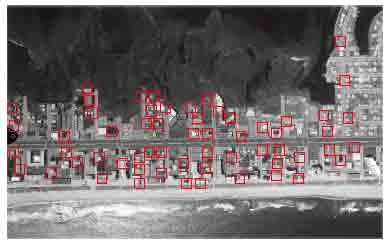
Figure 4.1 The test area and the distribution of the surface measurements
The following common parameters are used in this test: (S.D. Stands for Standard Deviation)
Focal length of the camera = 0.152764m;
S.D. of photo point measurement = 7 micrometers;
S.D. of surface points in X component = 0.07m;
Y=0.07m;
Z=0.12m.
Variance component of photo measurement = 1;
surface points = 1.
Table 4.1 Accuracy assessment
{ X0, Y0, Z0, w, j, K}: exterior orientation parameters;
{X, Y, Z} object point coordinates
Positional unit: meter; Angular unit: radian;
RMSE (Root Mean Square Error)
The adjustment results shown as in Table (4.1) lead to the following observations: The system proves itself workable by obtaining favorable accuracy both for exterior orientation parameters and object points coordinates. Note that again, the system works without the necessity of employing control points, the ingredient of indispensable for traditional aerial triangulation. Besides, the seemingly weak geometry with the available features within the narrow strip, as shown in Figure 4.1, does not prevent the system from finding satisfactory solution. It is obvious that the proposed model suggests its robustness and suitability for integrating surface estimation into aerial triangulation.
5. Conclusions
Aerial triangulation can be performed using the control surface rather than the control points, thus no identification of measured surface points with respect to their object truth is necessary. The control surface hypothesizing planes (first-order surface) in the object space may seem to oversimplify the surface at the first glance. Yet with increasingly available surface collectors, such as laser range finder and INSAR, the denser surface points data set would come into application field inevitably in the nearest future. Thus the available surface information would be analyzed in a more local scale in which the first-order surface, namely the plane, seems to be the most likely shape among all the others. Furthermore, for the residential area where artificial features dominate, the surfaces of the buildings including the roofs and the side walls, the surfaces of the road and many other man-made constructions provide abundant plane-like features not only in number but also in orientation, the proposed model shows its potential for the application in this area.
The proposed model solves not only the newly added object points via photogrammetric methods but also has the surface points adjusted through the registration of points from the photo space onto the object space. Thus the combined data set, the solved object points and the adjusted surface points together with their variance and covariance matrix [Jaw, 1999], would provide a better surface description for the task of surface analyses or surface reconstruction especially when image matching is to be exploited for the thorough surface generation. It is this author’s strongest emphasis for the contribution of this study on getting better estimation of the object space as a whole instead of watching out for every single point and/or the exterior orientation parameters.
Last but not least, the plane hypotheses and confirmation in the proposed model need no gridded DEM or special structure of surface points as a prerequisite, thus the original data set without being filtered or interpolated can be directly input to the system for the preservation of the firsthand accuracy.
References
Abstract
With the increased availability of surface-related sensors, the collection of surface information becomes easier and more straightforward than ever before. Thus, the integration of surface information into the photogrammetric workflow, the task which has been long time interesting as well as challenging, is gaining focus again within the photogrammetric community. In this paper, the author proposes a model in which the surface information is integrated into the aerial triangulation workflow by hypothesizing plane observations in the object space, the estimated object points via photo measurements (or matching) together with the adjusted surface points would provide a better point group describing the surface. Apart from releasing aerial triangulation from the necessity of identifying control points in the object space, the proposed algorithms require no special structure of surface points and involve no interpolation process. The proposed system is proven workable having data collection in the photogrammetric laboratory.
1. Introduction
More and more surface related sensors, such as airborne laser range finder, INSAR (INterferometric Synthetic Aperture Radar) with tightly integrated on-board GPS/INS system became commercially available during the last decade. By that, the booming research and applications mainly in generating elevation information for the area of interest and scene analyses, especially for the buildings in residential areas have been, among others, promising an era of sensors in which the collection of surface information becomes easier and more straightforward than ever before. Besides, due to the state-of-the-art of the sensor integration technique [Schwarz, 1995], the accuracy of the analyzed surfaces via airborne laser scanning system proves competitive with the scenario where a well-controlled data set and careful measurements by the operator are the necessities for the accuracy typical in traditional photogrammetric production line. Thus, how would photogrammetrists consider this newly available technique and its seemingly favorable data set apart from the aforementioned interests? One of the attractive thoughts follows: Can aerial triangulation by taking photo measurements benefit from this sensor dominant era and do a better job for the task of the surface reconstruction and how? These questions led the author into this study.
This very same idea and attempt had been carried out a decade ago at the Technical University of Munich, Germany, conducted by Ebner [Ebner/Strunz,1988][ Ebner et al., 1991][ Ebner/Ohlhof, 1994] even when the laser range data did not yet come to applications. Their algorithms focused mainly on the satisfaction of accuracy for the middle and small scale photogrammetry by minimizing the differences between the heights of the object-to-be-solved and the interpolated heights (bilinear interpolation) via the surrounding surface points, DEMs (Digital Elevation Models) in their case, as constraints. In this study, without interpolation on the surface points and requiring no special structure of the surface points, the author exploits different algorithms by hypothesizing planes (also called “control surface” in this paper) and assessing the uncertainties via checking the fitting planes with local surface points; the minimization takes distances along the surface normal as the target function when formulating the surface constraint.
The rest of this paper consists of the following: Section two introduces the surface constraint with formulating its mathematical as well as stochastic model. The integration of surface constraint into aerial triangulation is explained in section three. Section four demonstrates the experimental test in the photogrammetric laboratory together with the accuracy (root mean square error) report and the analyses. Section five concludes this study by giving some observations of this research from this author’s perspective.
2. Model Formation of the Surface Constraint
2.1 The First– Order Surface (Plane) Equation:
Mathematically, three points, let’s say and P1(X1, Y1, Z1), P2(X2, Y2, Z2) and P3(X3, Y3, Z3)define a plane. The plane equation with c b and a, being the function of coordinate components of three points can be seen as equation (2.1).
aX + bY + cZ + d =0 (2.1)
To calculate the distance along the surface normal between a point Pi(Xi, Yi, Zi) and the plane aX + bX +cZ + d =0, one could use equation (2.2) shown as below,
2.2 The Surface Constraint:
Analytically, if a point is known to lie on the known plane, equation (2.1) would be automatically realized. A direct result of that is that the distance calculated by using equation (2.2) would end up with zero.
Realistically, due to the measuring errors of the employed instrument, the physical truth of the plane could hardly be found by the collected data. Thus if the points are judged to lie on the known plane, one would compromise the observations by minimizing the distances along the normal, shown as equation (2.3), such that the imperfection of the measurements and the overall registration of the data set could be taken into account in an optimal way towards the solution. By that, the author proposes an algorithm in which the plane is hypothesized in the object space and confirmed by the surface points, thus forming the surface constraint into the adjustment for simultaneously determining the object points and the exterior orientation parameters via aerial triangulation procedures.
2.3 The Functional as well as the Stochastic Model of the Surface Constraint
The symbols in equation (2.3) are classified into two groups, namely the observations and the unknowns. For this study, what is known are the surface points while those points Pi(Xi, Yi, Zi) considered to lie on the planes are the unknowns through the photogrammetric measurements. One, therefore, is able to formulate functional model as well as stochastic model of the control surface constraint shown as equation (2.4)
 |
(2.4) |
 |
where
n : the number of object points from the photo measurements;
m : the number of surface constraints;
q :the number of registered surface points;
w: the discrepancy ((lio derived with the approximations of the unknowns and the observations;
y : the observations of the known surface points;
B : the coefficients of partial derivatives with respect to the surface points;
A : the coefficients of partial derivatives with respect to the unknowns of the object points( may include 0mx3(n-m) for those object points unable to find registered surface planes);
x :the unknowns of the object points ;
e :the random errors of the surface points;
S0 : the dispersion matrix of the surface points;
Po : the weight matrix of the surface points;
s02 : the variance component of the surface points;
Yet from the prediction point of view, the closer the unknown object point is to the registered surface point, the more reliable the constraint information would become. The error-propagated uncertainty assessment of the surface constraint based on the aforementioned model does not find itself the same conclusion. Therefore a modification of the stochastic model compromising the likely conflict due to the imperfect analytical model is needed [Jaw, 1999]. The modification performs in a way such that the x00, as shown below, reflects the deviation of the plane formation by three surface points from the fitting plane by all the neighboring surface points. We therefore come to the modified model as follows,
 |
(2.5) |
 |
where
Poo : the weight matrix of the added uncertainty;
stands for the weight matrix of surface
constraint after the modification; Due to the restricted space in this paper, the author encourages the interested readers refer [Jaw, 1999] for more detailed explanation of the model modification.
3. Control Surface in Aerial Triangulation
With the formulation of surface constraint model, the photogrammetric measurements can be joined into the system performing the aerial triangulation task. The combined model is expressed as below,
 |
(3.1) |
 |
where
y1 : increments of the photo observations, namely the difference between the original observations and the derived observation via the approximations;
k : number of the photo point measurements;
p : number of the photos ; n : number of the object points to be determined;
A11 : the coefficient matrix derived from taking partial derivatives with respect to the exterior orientation parameters;
A12 : the coefficient matrix derived from taking partial derivatives with respect to the object point coordinates;
x
x
e1 : the random errors of the photo point measurements;
s012 : the variance component of the photo point measurements;
P1 : the weight matrix of the photo point measurements;
w : the discrepancy of the surface constraint;
A22 is A in equation (2.4) plus 0mx3(n-m) for those object points unable to find registered surface planes;
m : number of the surface constraints;
e2 : the random errors of the registered surface points;
s012 : the variance component of registered surface points;
: the weight matrix of the modified
surface constraints; Thus the redundancy of the system is calculated as
r=(2k+m)-(6p+3n) (3.2)
4. Experimental Results and Analyses
The author conducted an experiment using an analytical plotter for collecting both the ground truth and the measuring data. The measurements involving 4 consecutive stereomodels were performed by the Zeiss C120 Analytical Plotter in the photogrammetric laboratory at the Department of Civil and Environmental Engineering and Geodetic Science, the Ohio State University. The photographs with about 1/4000 scale were taken at Ocean City, Maryland in April, 1997. The area of interest has been aerially triangulated by using highly accurate GPS site measurements as the control points. Accordingly, the author treats the exterior orientation parameters as the true values for the collection of the object points, then comparing them with the solved parameters in order to assess the empirical accuracy (root mean square error). The coverage of the test area and the measured plane features, as marked, can be seen in Figure 4.1.
Figure 4.1 The test area and the distribution of the surface measurements
The following common parameters are used in this test: (S.D. Stands for Standard Deviation)
Focal length of the camera = 0.152764m;
S.D. of photo point measurement = 7 micrometers;
S.D. of surface points in X component = 0.07m;
Y=0.07m;
Z=0.12m.
Variance component of photo measurement = 1;
surface points = 1.
Table 4.1 Accuracy assessment
| PARAMETERS | X0 | Y0 | Z0 | w | j | K | X | Y | Z |
| RMSE | 0.11 | 0.12 | 0.09 | 0.000136 | 0.000416 | 0.000212 | 0.133 | 0.057 | 0.072 |
{ X0, Y0, Z0, w, j, K}: exterior orientation parameters;
{X, Y, Z} object point coordinates
Positional unit: meter; Angular unit: radian;
RMSE (Root Mean Square Error)
The adjustment results shown as in Table (4.1) lead to the following observations: The system proves itself workable by obtaining favorable accuracy both for exterior orientation parameters and object points coordinates. Note that again, the system works without the necessity of employing control points, the ingredient of indispensable for traditional aerial triangulation. Besides, the seemingly weak geometry with the available features within the narrow strip, as shown in Figure 4.1, does not prevent the system from finding satisfactory solution. It is obvious that the proposed model suggests its robustness and suitability for integrating surface estimation into aerial triangulation.
5. Conclusions
Aerial triangulation can be performed using the control surface rather than the control points, thus no identification of measured surface points with respect to their object truth is necessary. The control surface hypothesizing planes (first-order surface) in the object space may seem to oversimplify the surface at the first glance. Yet with increasingly available surface collectors, such as laser range finder and INSAR, the denser surface points data set would come into application field inevitably in the nearest future. Thus the available surface information would be analyzed in a more local scale in which the first-order surface, namely the plane, seems to be the most likely shape among all the others. Furthermore, for the residential area where artificial features dominate, the surfaces of the buildings including the roofs and the side walls, the surfaces of the road and many other man-made constructions provide abundant plane-like features not only in number but also in orientation, the proposed model shows its potential for the application in this area.
The proposed model solves not only the newly added object points via photogrammetric methods but also has the surface points adjusted through the registration of points from the photo space onto the object space. Thus the combined data set, the solved object points and the adjusted surface points together with their variance and covariance matrix [Jaw, 1999], would provide a better surface description for the task of surface analyses or surface reconstruction especially when image matching is to be exploited for the thorough surface generation. It is this author’s strongest emphasis for the contribution of this study on getting better estimation of the object space as a whole instead of watching out for every single point and/or the exterior orientation parameters.
Last but not least, the plane hypotheses and confirmation in the proposed model need no gridded DEM or special structure of surface points as a prerequisite, thus the original data set without being filtered or interpolated can be directly input to the system for the preservation of the firsthand accuracy.
References
- Ebner, H., Strunz, G., 1988. Combined Point Determination Using Digital Terrain Models as Control Information. International Archives of Photogrammetry and Remote Sensing , ISPRS XVIth Congress, Vol. 27 Part B11, Kyoto, pp. III/578-III/587.
- Ebner, H., Strunz, G., Colomina, I., 1991. Block Triangulation with Aerial and Space Imagery Using DTM as Control Information. ACSM-ASPRS Auto-Carto 10, Annual Convention, Technical Papers, Baltimore, March 25-29, Vol. 5, pp. 76-85.
- Ebner, H., Ohlhof, T., 1994. Utilization of Ground Control Points for Image Orientation without Point Identification in Image Space. International Archives of photogrammetry and Remote Sensing, ISPRS Commission III Symposium, Munich, Sep, Vol. 30, Part 3/1, pp. 206-211.
- Jaw, J.J., 1999. Control Surface in Aerial Triangulation. Ph.D. dissertation, The Dept. of Civil and Environmental Engineering and Geodetic Science, The Ohio State University, Columbus, Ohio.
- Schwarz, K., 1995. Integrated Airborne Navigation Systems for Photogrammetry. Photogrammetric Week’95 Stuggart, Fritsch/Hobbie(Eds.), pp. 139-153.