| GISdevelopment.net ---> AARS ---> ACRS 1998 ---> Water Resources |
Remote Sensing of SST Around
the Outfall of a Power Plant from LANDSAT and NOAA Satellites
Ruo-Shan
Tseng
Departemtn of Marine Resources
National Sun Yat-sen University
Kaohsiung, Taiwan 804
Tel: 886-7-5252000 ext 5033 Fax: 886-7-5255033
E-mail: mailto:rstseng%20@mail.nsysu.%20edu%20tw
AbstractDepartemtn of Marine Resources
National Sun Yat-sen University
Kaohsiung, Taiwan 804
Tel: 886-7-5252000 ext 5033 Fax: 886-7-5255033
E-mail: mailto:rstseng%20@mail.nsysu.%20edu%20tw
Satellite data from Landsat Thematic Mapper (TM) and NOAA Advanced Very High Resolution Radiomether (AVHRR) were used to derive sea surface temperature (SST) in coastal waters of Hsinta that receive cooling effluent from a power plant. Ground truth (GT) temperature measured simultaneously from a ship as Landsat passed were applied in this paper to improve the atmospheric correction process for monitoring SST. Local radiosonde measurements, used in Lowtran7 adjustments for atmospheric effects, produced corrected ocean surface radiances and atmospheric transmittances. Secondly, a scheme combining NOAA-AVHRR and Landsat-TM data was used to derive SST. The advantage of this scheme is that no atmospheric correction process is required. Both methods showed good agreement between the GT and satellite-derived SST for thermal plume of Hsinta power plant.
Introduction
The capability of the TM flown on Landsat 4 and 5 to estimate the SST for the purpose of monitoring thermal plumes produced by power plants has been demonstrated by Gibbons and Wukelic (1989) and Liu and Kuo (1994). Both studies used the thermal band 6) data combining with some sorts of atmospheric processes which require local radiosonde measurements used in LOWTRAN 6 or 7 adjustments. Although the spatial resolution of the thermal band is only 120m, it can provide some insight into the distribution of SST in coastal waters that receive cooling effluent from a power plant. On the other hand, multi-channel sea surface temperature (MSST) techniques have been commonly used for the AVHRR onboard NOAA series satellites for over twenty years, and the root mean square differences of about 0.6°C were found between satellite and in situ data from drifting buoys (Strong and McClain, 1984). In spite of this high accuracy of SST measurements by the AVHRR, its spatial resolution of 1.1 km is too rough for thermal plume analysis in a relatively small area.
An attempt was made in this paper to incorporate both TM and AVHRR data to monitor power plant thermal discharges. The main idea was to make use of the high-resolution advantage or TM data and the high-accuracy advantage of AVHRR data. A simple scheme was then developed to derive the SST without going through the atmospheric correction processes.
Ground Truth and Satellite Data
The study area for this research is at Hsinta power plant which is located in the southwestern Taiwan coast (Fig. 1). The cooling water discharges via an open channel into shallow water of a coastal embayment south of Hsinta harbor that connects to deeper water in the open ocean. In order to validate and compare with the satellite results, one field trip was made to measure the surface-layer water temperature by a ship when the Landsat overpassed this study area at 09:40 local time on 27 June 1996. The temperature of the upper 1m of the sea surface was measured with a conductivity-temperature-depth recorder (CTD), which has an error of ±0.01°C. Ship's loacation was determined by a DGPS, which has an error of within 3 m. The sampling points of SST were centered at the plant outfall and spreaded radially out to a distance of about 2 km. Radiosonde data acquired at the nearby Tungkang readiosonde station were obtained for the overflight data. The vertical measurements of atmospheric pressure,temperature, and dew point, from sea level to 24 km, were used as input to LOWTRAN to correct atmosphere scattering and absorption. The level 10, digital data of TM acquired by the National Central University were obtained for the data of June 27, 1996. Digital AVHRR data of NOAA-12 and NOAA-14 satellites were aquired by our own HRPT receiving station situated at the National sun yat-sen University. A software of MAPIX-OCEAN was used to read the digital data and calculate the SST according to the MCSST equations.
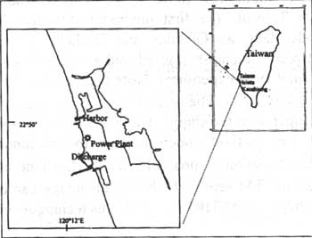
Fig. 1 The site of Hsinta Power Plant
Data processing Procedures
Two methods were applied to the TM data for coastal thermal plume analysis. The first method is to calculate the corrected radiance and temperature by putting radiosonda data into-LOWTRAN 7 to correct for atmospheric effects. The shoreline can be determined from the band5 digital data, because the reflectance of solar energy in the near-IR band from the water surface is much lower than from the land surface. Fig.2 shows the shoreline determination of the studied site using contour lines of band 5 digital counts of 20. Note that an area of the size 70 x 70 pixels was selected for data analysis in this study. The Hsinta harbor, power plant and the outfall can all be clearly identified in Fig. 2 The second method incorporates AVHRR data into TM temperature of each pixel near thermalplume deviates markedly from the ground truth due to the atmospheric effect, they still exhibit a correct spatial distribution of temperature. The spatial distribution characteristics of temperature can be represented by a simple dimensionless matrix P(i), i.e.,
Where Tb(i)is the uncorrected brightness temperature of the ith pixel,
 b is the average of
brightness temperature of all pixels in the selected area. Since the
AVHRR-derived SST has been thermal plume can be obtained by
2)
b is the average of
brightness temperature of all pixels in the selected area. Since the
AVHRR-derived SST has been thermal plume can be obtained by
2) Where
is the average of AVHRR-derived SST of All
pixels in the selected area, T(i) is the corrected SST of the ith pixel.
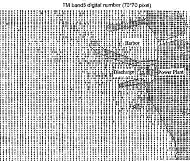
Fig.2 Shoreline determination using Landsat-5 TM band 5. Solid lines indicate contour lines of digital counts with value of 20.
Results and Discussion
Table 1 shows the uncorrected and corrected (after applying LOWTRAN 7 process) radiance and brightness temperature for the TM thermal IR band. One can find that there are differences of 9 to 10°C between ship-measured SST and the uncorrected brightness temperature when the atmospheric effects were negligible. This is not uncommon in moist summer conditions at southern Taiwan (Liu and Kuo, 1994). After applying the atmospheric correction process, the radiance increased significantly and the mean and RMS of the difference between the GT and corrected SST reduced to -0.04°C and 1.22°C, respectively. The difference between the GT and corrected SST at near the outfall location is only 0.71°C. A correlation coefficient between the GT and corrected SST for all the 33 data points in Table 1 was found to be 0.78. Fig. 3 is a color-coded plot showing the distribution of estimated TM-derived SST on 27 June 1996 near the Hsinta power plant. The thermal plume is a small structure on the larger ocean environment, and the discharged water appeared to disperse to the south. This feature is also consistent with the ship-measured SST (not shown here).
| Tu | GT | DTu=Tu-GT | Ru | Rc | Tc | DTc=Tc-GT | Tu | GT | DTu-GT | Ru | Rc | Tc | DTc=Tc-GT | |
| 21.75 | 28.97 | -7.22 | 0.86 | 0.98 | 30.86 | -1.89 | 21.30 | 30.26 | -8.96 | 0.85 | 0.96 | 29.86 | 0.40 | |
| 21.30 | 30.14 | -8.84 | 0.85 | 0.96 | 29.86 | 0.28 | 21.30 | 30.05 | -8.75 | 0.85 | 0.96 | 29.86 | 0.19 | |
| 21.30 | 30.03 | -8.73 | 0.85 | 0.96 | 29.86 | 0.17 | 21.75 | 33.11 | -11.36 | 0.86 | 0.98 | 30.86 | 2.25 | |
| 21.30 | 29.87 | -8.57 | 0.85 | 0.96 | 29.86 | 0.01 | 22.20 | 33.13 | -10.93 | 0.86 | 0.99 | 31.84 | 1.29 | |
| 21.30 | 29.58 | -8.28 | 0.85 | 0.96 | 29.86 | -0.28 | 23.08 | 33.01 | -9.93 | 0.87 | 1.01 | 33.77 | -0.76 | |
| 22.60 | 30.51 | -7.91 | 0.87 | 1.00 | 32.72 | -2.21 | 22.20 | 30.88 | -8.68 | 0.86 | 0.99 | 31.84 | -0.96 | |
| 23.08 | 30.54 | -7.46 | 0.87 | 1.01 | 33.77 | -3.23 | 22.64 | 31.57 | -8.93 | 0.87 | 1.00 | 32.81 | -1.24 | |
| 22.64 | 34.59 | -11.95 | 0.87 | 1.00 | 32.81 | 1.77 | 22.64 | 32.56 | -9.92 | 0.87 | 1.00 | 32.81 | -0.25 | |
| 23.53 | 34.42 | -10.89 | 0.88 | 1.03 | 34.75 | -0.33 | 21.75 | 32.29 | -10.54 | 0.86 | 0.98 | 30.86 | 1.43 | |
| 23.53 | 34.16 | -10.63 | 0.88 | 1.03 | 34.75 | -0.59 | 21.75 | 30.08 | -8.33 | 0.86 | 0.98 | 30.86 | -0.78 | |
| 23.97 | 36.43 | -12.46 | 0.88 | 1.04 | 35.71 | 0.72 | 21.30 | 30.18 | -8.88 | 0.85 | 0.96 | 29.86 | 0.32 | |
| 23.53 | 35.09 | -11.56 | 0.88 | 1.03 | 34.75 | 0.34 | 21.75 | 31.50 | -9.75 | 0.86 | 0.98 | 30.86 | 0.64 | |
| 23.08 | 35.43 | -12.35 | 0.87 | 1.01 | 33.77 | 1.66 | 22.64 | 31.81 | -9.17 | 0.87 | 1.00 | 32.81 | -1.00 | |
| 22.20 | 34.36 | -12.16 | 0.86 | 0.99 | 31.84 | 2.52 | 22.20 | 32.54 | -10.34 | 0.86 | 0.99 | 31.84 | 0.70 | |
| 21.75 | 29.92 | -8.17 | 0.86 | 0.98 | 30.86 | -0.94 | 22.20 | 32.02 | -9.82 | 0.86 | 0.99 | 31.84 | 0.18 | |
| 21.75 | 30.10 | -8.35 | 0.86 | 0.98 | 30.86 | -0.76 | 22.20 | 31.56 | -9.36 | 0.86 | 0.99 | 31.84 | -0.28 | |
| 21.75 | 30.24 | -8.49 | 0.86 | 0.98 | 30.86 | -0.62 | ||||||||
| mean(DTc)=-0.04°C | RMS(DTc)= 1.22°C | |||||||||||||
Table 1. Uncorrected and corrected (after applying LOWTRAN 7 process) spectral radiances and temperature compared with ground truth (27 June 1996).
Tu: Uncorrected temperature (°C) Gt: ground truth (°C) Ru: Uncorrected radiance (mWcm-2 mm-1 sr-1)
Tc: corrected temperature (°C) Rc: corrected radiance (mWcm-2 mm-1 sr-1)
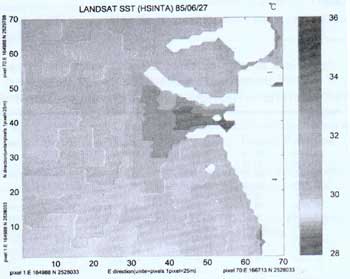
Fig.3 SST image in which atmospheric effects were corrected for using LOWTRAN (27 June 1996)
The AVHRR data of 13:00 27 June 1996 were used in the second method. According to the data processing procedures, 4 AVHRR pixels corresponding to the same locations of the 70x 70 TM pixels were selected for the studied site. The AVHRR-derived SST of these four pixels is 31.1°C, 31.52°C, 33.7°C and 34.42°C, respectively. The TM-derived brightness temperature is thus modified by the average temperature of these four pixels. Table 2 shows the GT and corrected (after applying AVHRR-data correction process) SST for the TM thermal IR band. One can see that the mean and RMS of the difference between the GT and corrected SST was found to be 0.86, which indicates a slightly better effect of correction than the first method. However, the difference between the GT and corrected SST at near the outfall location is 1.51°C, which is greater than the first method. Fig. 4 is a color-coded plot showing the distribution of estimated TM-derived SST on 27 June 1996 near the Hsinta power plant. The distribution and dispersing of the thermal plume are similar to Fig. 3, but the maximum temperature at the outfall is somewhat lower.
Concluding Remarks
Two methods were applied to the Landsat-TM data in determine the SST around the outfall of a power plant at Hsinta, southern Taiwan. The first method is through the atmospheric correction process using radiosonde data, as Gibbons and Wukelic (1989) suggested. It was found that the RMS error between the ship-measured and satellite-derived SST using this method was 1.22°C during the 27 June 1996 experiment. Note that results of the first method depend strongly on the quality of radiosonde data. The second method incorporates AVJRR data into TM data with a simple matrix operation technique. The RMS error of SST difference was found to be 1.18°C . However, this method underestimated the maximum temperature near the outfall for about 2°C. This deviation is probably due to the inherent disadvantage of poorer resolution of AVHRR than the TM sensor. If this disadvantage can be improved by a better registration of pixel locations between AVHRR and TM, this technique will become more feasible in the future.
Acknowledgemtn
This work was partly supported by the National Science Council of the Republic of China under Grant NSC 85-2611-P-110-005.
Reference:
- Gibbons, D.E. and G.E. Wukelic, 1989, Application of Landsat Thermatic Mapper Data for Coastal Thermal Plume Analysis at Diablo Canyon, Photogrammetric Engineering and Remote Sensing, 55(6): 903-909.
- Liu, G.-R. and TH.-H. Kuo, 1994, Improved Atmospheric Correction Process in Monitoring SST Around the outfall of Nuclear Power Plant, Int. J. Remote Sensing, 15(13); 2627-2636.
- Strong, A.E. and E.P. McClain, 1984, Improved Ocean Surface Temperatures from Space Comparisons with Drifting buoys, Bulletin American Meteoro. Society, 65(2) 138-142.
| Ts : satellite estimated SST (°C) | Tg : ship-measured SST (°C) | |||||||||||||||||||||||||||||||||||||||||||||||||||||||||||||||||||||||||||||||||||||||||||||||||||||||||
|
| |||||||||||||||||||||||||||||||||||||||||||||||||||||||||||||||||||||||||||||||||||||||||||||||||||||||||
| mean(Ts-Tg)=0.3152°C | RMS(Ts-Tg)=1.18°C |
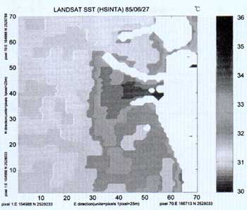
Fig 4. SST image combining AVHRR and TM data (27 June 1996)