| GISdevelopment.net ---> AARS ---> ACRS 1998 ---> Water Resources |
Reservoir Water Quality
Monitoring Using Landsat TM Images and Indicator Kriging
Cheng, Ke-Sheng, Lei, Tsu-Chiang, and Yeh, Hui-Chung
Agricultural Engineering Department, National Taiwan Unversity
1,Roosevelt Rd. Sec. 4.10617, Taipei, Taiwan, R.O.C.
Tel & Fax : (886)-2-2366-1568
E-mail :hcyhfc@ms22.hinet.net
Cheng, Ke-Sheng, Lei, Tsu-Chiang, and Yeh, Hui-Chung
Agricultural Engineering Department, National Taiwan Unversity
1,Roosevelt Rd. Sec. 4.10617, Taipei, Taiwan, R.O.C.
Tel & Fax : (886)-2-2366-1568
E-mail :hcyhfc@ms22.hinet.net
Abstract
Landsat TM images were used to study the trophic states of Te-Chi Reservoir located in central Taiwan. Water quality parameters such as total phoshate, ChlorophyII a concentration and secchi disk depth are found highly correlated with spectral parameters derived from Landsat TM images. Carlson trophic state index is adopted for evaluation of reservoir trophic states. The reservoir trophic states determined from field data and from satellite image are highly consistent, indicating great potential of using satellite image for reservoir water quality investigation.
Introduction
Many reservoirs in Taiwan have been found to receive significant pollutant loading from their upstream watersheds. Wide usage of agricultural pesticides and fertilizers, inappropriate landuse management high intensity rainfall and steep-slope farming are major factors that contribute to the degradation of reservoir water quality. Several jurisdictional agencies routinely collect water samples at channel inlets to the reservoir and at several reservoir cross sections. However, the vast coverage of reservoir water body makes it difficult to evaluate the trophic state of the reservoir as a whole. Also , a dense water quality monitoring network is not cost effective. In recent years have had growing interests in evaluating lake or reservoir water quality using remote sensing images. Lillesand et al. (1983), Lavery et al. (1993), Tassan (1993) and She et al. (1996) established different regression models for water quality parameters using Landsat TM images. We believe that these established regression models are at best localized models since changes in physiographic environment and geographic loacation have significant impact on algae production and incidental intensity of spectral bands.
Environmental impact assessment may require information about areas which have higher possibility of excessive pollution. Technique of spatial statistics such as indicator krging is useful for this purpose and is also employed in this study to delineate the boundaries for areas of high pollution potential.
Study site and data set
Te-Chi Reservoir located in Central Taiwan is selected for this study. Two types of data are used in this study: 1) Landsat TM images (TMI ~ TM4) collected on 8/31/1993, 10/5/1994. 1/9/1995 and 7/22/1996, and (2) water quality data collected by jurisdictional agencies. Exact location of water sampling were determined by using a GPS system in the field. Figure 1 illustrates the locations of water sampling. A total of 25 water quality parameters were analyzed from these samples, however, parameters needed for Carlson trophic state index (CTSI) calculation, i.e. total phosphate (TP), Chlorophyll-a concentration (Chla) and secchi disk depth (SDD), were only available at five locations, S-6, S-18, S-28,S-39 and R-4 (Figure 1).
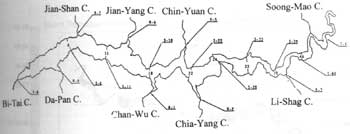
Figure 1 The river of Te-Chi Reservoir
Trophic states and Carlson trophic state index The water quality status, i.e. the tophic state, of large waterbodies like lakes and reservoirs is usually classified into three categories: oligotrophication, mesotrophication, and eutrophication. As the nutrients increase in the waterbodies, algae production increases and eutrophication state gradually develops. Carlson trophic state index (Carlson, 1977) is a combinatorial index that considers the total phosphate, ChlorophyII-aconcentration and secchi disk depth in reservoirs and lakes. The following equations are used for CTSI calculation:
A waterbody is in oligotrophic, mesotrophic or eutrophic state if CTSI < 40, 40 £ CTSI < 50, or 50 £ CTSI.
Reservoir trophic states evaluation using TM images
As we have mentioned, empirical relations between water quality parameters and remote sensing spectral parameters are localized, thus breakpoint regression analysis is used in this study to establish leash-squares relations between many combination foram of TM1 through TM4 and each of the three water quality parameters, TP, Chla and SDD. The following regression models give best estimates and are then used for CTSI calculation:
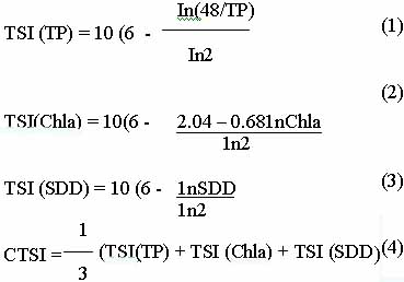
Estimates from the above equations are then substituted into Eq. (4) to calculate the Carlson index for every pixel in the reservoir. Figures 2 and 3 illustrate the spatial variation of trophic state in the reservoir on August 31, 1993 and January 9, 1995. It is seen clearly that upstream channel at the northeast corner has the worst water quality states. This is not unexpected as the channel receives sediments and nutrient output from a major vegetable and fruit production zone. Other areas in the vicinities of channel inlets also show higher values of CTSI.
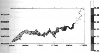
Figure 2 The spatial variation CTSI on Aug. 31 1993
Figure 3 The spatial variation CTSI on Jan. 9 1995
Identification of excessive pollution regions indicator krging
In light of the environmental impact assessment, it often desires to know areas of excessive pollution and delineate their boundaries for further regulatory or remedy actions. Identification of excessive pollution areas is based on the concept of higher probability of exceedance, say 0.8 for example, with respect to a predetermined and meaningful threshold. In this study the threshold is chosen at CTSI = 55 and areas with exceeding probability greater tan 0.8 are considered excessive pollution regions.
Indicator is one of the many geostatistical estimation methods. Unlike the most commonly used ordinary kriging method which gives estimates of interested parameter at unsampled locations, indicator kriging estimates the global or local distribution of the interested parameter. Several cutoff values of the interested parameter, say Z is transformed into either 1 or 0, i.e.
Where Zc is the cutoff Value Zj is the observed values of Z, is the total number of samples and Ij is called the indicator variable.
In geostatistics, the spatial variation of a random variable Z is characterized by a variogram function defined as:
gz(h) =
1/2[z(x+h)-z(x)]2
Where z(x) represents the value of Z at the location x. For indicatior kriging, variograms of indicator variables corresponding to different cutoff values must be established first and then global or local cumulative distribution function of Z can be estimated by using these indicator variograms. Readers are referred to Journal and Juijbgrets (1978) and Isaaks and Srivastave (1989) for details of ordinary and indicator kriging.
Using CTSI = 60 as cutoff value and applying indicator kriging to previously estimated CTSI (Figure 2), we identify the areas of excessive pollution for 8/31/1993 image (Figure 4). These are areas that may require remedy actions.
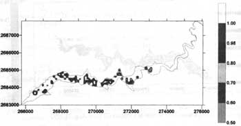
Figure 4 The spatial variation Indicator Kriging map on Aug. 31 1993.
Conclusions
We gratefully acknowledge the support of Water Resources Department, Ministry of Economic Affairs (WRD - MOEA) in field data collection. This study would be possible without their support.
References
Landsat TM images were used to study the trophic states of Te-Chi Reservoir located in central Taiwan. Water quality parameters such as total phoshate, ChlorophyII a concentration and secchi disk depth are found highly correlated with spectral parameters derived from Landsat TM images. Carlson trophic state index is adopted for evaluation of reservoir trophic states. The reservoir trophic states determined from field data and from satellite image are highly consistent, indicating great potential of using satellite image for reservoir water quality investigation.
Introduction
Many reservoirs in Taiwan have been found to receive significant pollutant loading from their upstream watersheds. Wide usage of agricultural pesticides and fertilizers, inappropriate landuse management high intensity rainfall and steep-slope farming are major factors that contribute to the degradation of reservoir water quality. Several jurisdictional agencies routinely collect water samples at channel inlets to the reservoir and at several reservoir cross sections. However, the vast coverage of reservoir water body makes it difficult to evaluate the trophic state of the reservoir as a whole. Also , a dense water quality monitoring network is not cost effective. In recent years have had growing interests in evaluating lake or reservoir water quality using remote sensing images. Lillesand et al. (1983), Lavery et al. (1993), Tassan (1993) and She et al. (1996) established different regression models for water quality parameters using Landsat TM images. We believe that these established regression models are at best localized models since changes in physiographic environment and geographic loacation have significant impact on algae production and incidental intensity of spectral bands.
Environmental impact assessment may require information about areas which have higher possibility of excessive pollution. Technique of spatial statistics such as indicator krging is useful for this purpose and is also employed in this study to delineate the boundaries for areas of high pollution potential.
Study site and data set
Te-Chi Reservoir located in Central Taiwan is selected for this study. Two types of data are used in this study: 1) Landsat TM images (TMI ~ TM4) collected on 8/31/1993, 10/5/1994. 1/9/1995 and 7/22/1996, and (2) water quality data collected by jurisdictional agencies. Exact location of water sampling were determined by using a GPS system in the field. Figure 1 illustrates the locations of water sampling. A total of 25 water quality parameters were analyzed from these samples, however, parameters needed for Carlson trophic state index (CTSI) calculation, i.e. total phosphate (TP), Chlorophyll-a concentration (Chla) and secchi disk depth (SDD), were only available at five locations, S-6, S-18, S-28,S-39 and R-4 (Figure 1).
Figure 1 The river of Te-Chi Reservoir
Trophic states and Carlson trophic state index The water quality status, i.e. the tophic state, of large waterbodies like lakes and reservoirs is usually classified into three categories: oligotrophication, mesotrophication, and eutrophication. As the nutrients increase in the waterbodies, algae production increases and eutrophication state gradually develops. Carlson trophic state index (Carlson, 1977) is a combinatorial index that considers the total phosphate, ChlorophyII-aconcentration and secchi disk depth in reservoirs and lakes. The following equations are used for CTSI calculation:
A waterbody is in oligotrophic, mesotrophic or eutrophic state if CTSI < 40, 40 £ CTSI < 50, or 50 £ CTSI.
Reservoir trophic states evaluation using TM images
As we have mentioned, empirical relations between water quality parameters and remote sensing spectral parameters are localized, thus breakpoint regression analysis is used in this study to establish leash-squares relations between many combination foram of TM1 through TM4 and each of the three water quality parameters, TP, Chla and SDD. The following regression models give best estimates and are then used for CTSI calculation:
| Chla | { | -152.86 + 631.12 (TM3 / TM2) - 170.38
(TM2 x TM3)/TM 1 + 438.45 TM4 / (TM2 + TM3) + 1.65(TM2 x TM3)/ TM 1
Chla< = 196.53 -3777.28 + 121160.98 (TM3 / TM2) - 2592.30 (TM2 x TM3) / TM 1 +2973.82 TM4 / (TM2 + TM3) + 23.16 (TM2 x TM3)/TM 1 Chla > 196.53 (5) |
| TP | { | 386.10 + 332.44 TM2 + 4435.84 (TM2 /TM
1) +23.6.05 TM4 / (TM2 + TM3) - 756.74 TM2 / log (TM 1)
TP<=90.17 1014.84 - 445.07 TM2 - 14135.2 (TM2 / TM 1) -548.36 TM4 / (TM2 = TM3) + 1158.84 TM2 / log (TM 1) TP>90.17 (6) |
| log SDD | { | 0.66 + 0.45 TM4 / (TM3 + TM2) + 0.906
(TM3 x TM4) / (TM1 + TM2) - 0.05 TM3 / log (TM3) log SDD
<=0.15 -0.14 - 0.25TM4 / (TM3 + TM2)- 0.365 (TM3 x TM4) / (TM1 + TM2) + 0.082 TM3 / log (TM3) log SDD>0.15 (7) |
Estimates from the above equations are then substituted into Eq. (4) to calculate the Carlson index for every pixel in the reservoir. Figures 2 and 3 illustrate the spatial variation of trophic state in the reservoir on August 31, 1993 and January 9, 1995. It is seen clearly that upstream channel at the northeast corner has the worst water quality states. This is not unexpected as the channel receives sediments and nutrient output from a major vegetable and fruit production zone. Other areas in the vicinities of channel inlets also show higher values of CTSI.
Figure 2 The spatial variation CTSI on Aug. 31 1993
Figure 3 The spatial variation CTSI on Jan. 9 1995
Identification of excessive pollution regions indicator krging
In light of the environmental impact assessment, it often desires to know areas of excessive pollution and delineate their boundaries for further regulatory or remedy actions. Identification of excessive pollution areas is based on the concept of higher probability of exceedance, say 0.8 for example, with respect to a predetermined and meaningful threshold. In this study the threshold is chosen at CTSI = 55 and areas with exceeding probability greater tan 0.8 are considered excessive pollution regions.
Indicator is one of the many geostatistical estimation methods. Unlike the most commonly used ordinary kriging method which gives estimates of interested parameter at unsampled locations, indicator kriging estimates the global or local distribution of the interested parameter. Several cutoff values of the interested parameter, say Z is transformed into either 1 or 0, i.e.
| ij=( | 1 if zj£zc | j=1,2,...,n |
| 0 if zj> zc |
Where Zc is the cutoff Value Zj is the observed values of Z, is the total number of samples and Ij is called the indicator variable.
In geostatistics, the spatial variation of a random variable Z is characterized by a variogram function defined as:
Where z(x) represents the value of Z at the location x. For indicatior kriging, variograms of indicator variables corresponding to different cutoff values must be established first and then global or local cumulative distribution function of Z can be estimated by using these indicator variograms. Readers are referred to Journal and Juijbgrets (1978) and Isaaks and Srivastave (1989) for details of ordinary and indicator kriging.
Using CTSI = 60 as cutoff value and applying indicator kriging to previously estimated CTSI (Figure 2), we identify the areas of excessive pollution for 8/31/1993 image (Figure 4). These are areas that may require remedy actions.
Figure 4 The spatial variation Indicator Kriging map on Aug. 31 1993.
Conclusions
- We have established empirical relations between the three water quality parameters and spectral parameters of TM images. Using these equations, we are able to investigate the spatial variation of reservoir trophic state. However, it is important to recognize that as more water quality samples being collected, modification of these empirical relations maybe necessary.
- Indicator kriging is a useful tool for identifying excessive pollution regions. It has great potential of applications in environmental regulation or remediation since this type of applications usually have clearly defined and meaningful threshold values that can be used as cutoff values in indicator kriging.
We gratefully acknowledge the support of Water Resources Department, Ministry of Economic Affairs (WRD - MOEA) in field data collection. This study would be possible without their support.
References
- Carlson, R.E. (1977). A trophic state index for lakes. Limnol. Oceanog., Vol. 22, No.2, pp. 361~369.
- She, F., X. Li, Q. Cai and Y. Chen (1996), Quantitative anlysis on Chlorophyll-a concentration in Taihu Lake using Thematic Mapper data, J. of Lake Sciences, Vol. 8, No. 3 o
- Isaaks, E. and R. Srivastave (1989). An Introduction to Applied Geostatistics. Oxford University Press, New York.
- Journal, A. and C.J. Huijbgrets (1978). Mining Geostatistics. Academic Press, New York.
- Lavery, P., C. Pattiaratchi, A. Wyllie and P. Hick (1993). Water quality monitoring in estuarine water using the Landsat Thematic Mapper, Remote Sensing of Environment, Vol. 46, pp. 268-280.
- Lillesand, T.M., W.L. Johnson, R.L. Deueil, O.M. Lixdstrom and D.E. Meisner (1983). Use of Landsat data to predict the trophic state of Minnesota lakes, Photogrammetric Engineering & Remote Sensing, Vol. 49, No 2, pp. 219~229.
- Tassan, S. (1993). An improved in-water algorithm for the determination of chlorophyll and suspended sediment concentration from Thematic Mapper data in coastal waters. Int. J. Remote Sensing, Vol.14 No. 6 pp. 1221~1229.