| GISdevelopment.net ---> AARS ---> ACRS 1998 ---> Poster Session 3 |
Multi-model Histogram Linear
Contrast Stretching For Image Enhancement
P. Komonvipaht, K.
Wongsritong, F. Cheevasuvit, K. Dejhan, S. Chitwong, and S.
Mitatha
Faculty of Engineering, King Mongkut's Institute of Technology Ladkrabang
Bangkok 10520, Thailand.
E-mail: kcfusak@kmitl.ac.th
AbstractFaculty of Engineering, King Mongkut's Institute of Technology Ladkrabang
Bangkok 10520, Thailand.
E-mail: kcfusak@kmitl.ac.th
Image enhancement, modifying the value of picture elements, is a classical method for improving the visual perception. Therefore, the processed image is more suitable than the original image for some applications. The most well-known method is the histogram equalization because of its automatic procedure. However, the effect of brightness saturation will be appeared in some quasi-homogeneous region. This causes from the merging or adjacent gray levels process for flattening the global histogram. Not only some lower brightness will be grouped together but also some higher brightness in order to uniformize the histogram distribution. Unlike the method of histogram linear contrast stretching the new wide histogram dynamic range can be assigned directly from the original narrow histogram dynamic range. However, the histogram of an image can be composed of many models of histogram. Different modals can be represented with different objects. To enhance each modals of histogram independently, the obtained result image will get better visual perceptibility than the global enhancement. The standard deviation of each modals will be calculated and summed for providing the proportional of stretching range. The resultant image can be provided the higher efficiency in image segmentation or image classification. Therefore, this paper tries to carry out a method of the multi-modal histogram linear contrast stretching. As each modal of histogram can be detected by using the change of eight consecutive signs, each sign is obtained from the difference between two probabilities of adjacent gray level.
Introduction
A digital image is encoded the picture element with L bits, the gray level of brightness will be varied from 0 to 2L-1. The probability of each gray level is defined by the following equation;
P(rk) = nk/N (1)
Where rk is the kth gray level, nk is the number of pixel for the kth gray level and n is the total number of pixels in the image. The distribution of all gray level probabilities is called histogram. If a digital image has a narrow dynamic range of histogram, the image will give low contrast. So the different objects in the scene will have almost the same brightness. This will cause the difficulty in some applications such as an object identification, an object classification, and etc. To improve the contrast for the image enhancement, the methods of histogram modification are always employed to spread out the dynamic range. The most well-known method is histogram equalization. However, this method will be spread out the histogram and always reach the whitest and the blacked brightness. By consequently, the saturation of brightness will be appeared not only in quasi-homogeneous of low gray level but also in quasi-homogeneous of high-gray level. Unlike the method of histogram linear contrast stretching, the problem of brightness saturation can be avoided if the narrow range of original histogram is prosperously assigned to spread out.
Model detection
Since a histogram of image will be discontinued and fluctuated, therefore linear interpolation and smoothing method are applied to conquer these problems. For the smoothing procedure, nine consecutives of gray level probabilities are used to average. This average value is replaced by the central probability. The average value can be calculated as the following equation.
Pn(rk) = 1/9 9Si=1 p(rk-s+1) for 5<k<L-4 (2)
To obtain the break points for discriminating each modals in the histogram, the signs of two successive smooth probabilities will be calculated. The fluctuation of sign still exists. To smooth the sign, three consecutive signs will be considered for changing such as the following examples,
+ - + change to + + +
and - + - change to - - -
After the sign changing process is finished, the modal detection is applied. To carry out a break point for distinguishing two adjacent modals, the twelve consecutive signs are accounted. The break point is defined by these four negative signs followed by eight positive signs. So the break point is the point is the point that change from negative sign to positive sign.
Histogram linear contrast stretching
Since, the histogram can be composed of many modals which correspond to different objects in the image scene. To enhance each objects or to increase the contrast of the scene, each modals will be linearly stretched by using equation (3).
where xmin,k =
 - 2sk (4)
 and xmax,k =
- 2sk (5) and sk are the mean and standard deviation of
the kth modal respectively, xmin,k and xmax,k stand
for the original narrow dynamic range of kth modal. For the histogram with
p modals, the value of ymin,1 is set to 0 and the value of
ymax,p is set to 255. The width of the stretching range
(ymax,k - ymin,k) will be obtained by the
proportional of its standard deviation by using the following equation.
(ymax,k - ymin,k) = sk/sr x 256 (6)
where sr = pSk=1 sk (7)
Resultant
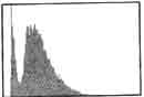
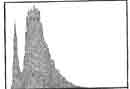
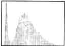
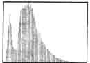
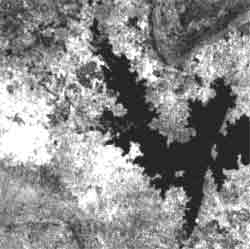
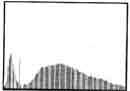
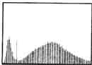
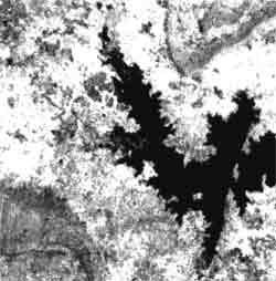
The three band satellite images as shown in Fig 1. is used as an example, and he Fig 2 is the corresponding histogram of each bands with images in Fig 1. For global histogram linear contrast stretching is applied to the histogram of Fig 2; the stretched histogram are obtained as shown in Fig. 3 and the corresponding result of colour image is presented in Fig. 4. While the Fig. 5 is manifested the result of the multi-modal histogram linear contrast stretching, the result of colour image obtained from the proposed method is demonstrated in Fig. 6. The comparisons of colour image in Fig. 4 and Fig. 6 are clearly shown that the proposed method gave a high contrast and the boundaries of each region in the image are clearly emphasized. Therefore, the process of image segmentation and classification can be efficiently achieved from the resutlful image.
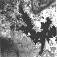 1(a) Red band |
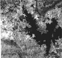 1(b)Green band |
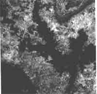 1(c)Blue band |
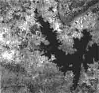 1(d)Colour image |
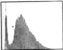 2(a) Histogram of red band |
 2(b) Histogram of Green band |
 2(c) Histogram of blue band |
 3(a) Histogram of red band |
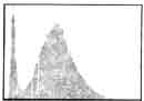 3(b) Histogram of green band |
 3(c) Histogram of blue band |
 |
 5(a) Histogram of red band |
 5(b) Histogram of green band |
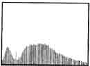 5(c) Histogram of blue band |
 |
Acknowledgements
The authors would like to think the National Research Council of Thailand (NRCT) for providing the satellite images and Miss Janira Jittaviriyapong for providing the manuscript. Miss Janjira is with the Department of Languages and Social Science, Faculty of Industrial Education, King Mongkut's Institute of Technology Ladkrabang, Bangkok, Thailand.
Reference
- John C. Russ, "The Image Processing Handbook, " 2nd Edition, IEEE Press, 1994,
- R. C. Conzalez and P. Wintz, "Digital Image Processing," 2nd Edition, Addison-Wesley Publishing Co., Reading, Massachusetts, 1987.
- M. A. Sid-Ahmed, "Image Processing :Theory, Algorithm & Architectures," McGraw-Hill International Editions, 1995.
- Y. T. Kim, "Contrast Enhancement using Brightness Preserving Bi-Histogram Equalization," IEEE Trans On Consumer Electronic, vol. 43, no. 1, pp. 1-8, Feb. 1997.