| GISdevelopment.net ---> AARS ---> ACRS 1998 ---> Poster Session 3 |
An Improvement of Geometric
Correlation of Satellite Image
Sompong Wisetphanichkij,
Kobchai Dejhan, Fusak Cheevasuvit, Somsak Mitatha and Somkid
Hanpipatpongsa
Faculty of Engineering and Research Center for Communication and Information Technique,
King Mongkut's Institute of Technology Ladkrabang, Ladkrabang,
Bangkok 10520, Thailand
Tel-: 66-2-3269967, 66-2-3269081, Fax : 66-2-3269086.
E-mail: kobchai@telean.telecom.eng.kmitl.ac.th
Chanchai Pienvijarnpong
National Research Council of Thailand,
MOS-I Receiving Ground Station,
Ladkrabang, Bangkok 10520, Thailand
Chatcharin Soonyeekan
Faculty of Engineering, Kasem Bundit University
Pattankaran Road, Klongton, Bangkok 10250, Thailand
Abstract Faculty of Engineering and Research Center for Communication and Information Technique,
King Mongkut's Institute of Technology Ladkrabang, Ladkrabang,
Bangkok 10520, Thailand
Tel-: 66-2-3269967, 66-2-3269081, Fax : 66-2-3269086.
E-mail: kobchai@telean.telecom.eng.kmitl.ac.th
Chanchai Pienvijarnpong
National Research Council of Thailand,
MOS-I Receiving Ground Station,
Ladkrabang, Bangkok 10520, Thailand
Chatcharin Soonyeekan
Faculty of Engineering, Kasem Bundit University
Pattankaran Road, Klongton, Bangkok 10250, Thailand
The geometric distortion of the satellite image can be occurred according to many reasons. It can be divided into systematic and non-systematic (or random) distortion. It is necessary to correct before using. The precision of geometric correction depends on the ground control points (GCPs). The noise is the satellite image may be generated from the interface or the blur according to the cloud coverage, thus it is difficult to assign the positions of GCPs. This paper presents a method to assign automatically the GCPs by using image registration method based on a sequential similarly detection algorithms (SSDAs) technique (statistic correlation measurement). This method used the sub-image around GCP from the improved image acting as prototype image to assign the positions of GCPs for the improving satellite image, the correlation will also be used in order to obtain the precision and accuracy.
1. Introduction
The geometric distortion in remotely sensed images come from two sources: the internal distortion caused by the sensor and the external distortion caused by the platform and the subjects
- Internal distortion (Systematic distortion)
Variations of beam width and sampling in the sensor (or radar). - External distortion (Non systematic distortion)
Variations of the location, altitude, attitude and speed of the platform, the relief and curvature of the ground surface and the earth's revolution.
- Image to map (grid) registration is used the topographic map as a reference
- Image to image registration that one image referred to as the reference image and assumed to be good quality, i.e., no cloud, contrast is good and geometrical distortion are negligible. The search (input) image, on the other hand, is relatively unknown quality. Some coverage fog/cloud may be present along the geometrical distortion.
Image to image registration is a procedure to determine the spatial best fit between two images that overlap the same scene. In the sake of two images for the same scene cannot be meaningfully compared. Several digital techniques have been used for registering imagery Principal among these are cross-correlation, normalized cross-correlation (Eq.1) and minimum distance criteria. Fast algorithms for determining translational difference between images have been developed in recent years for all techniques [1].
Where (j,k) are indices in a JxK point window area (W) that is located within an MxN point of search area (S)
Fig. 1 Relationship between search and window areas
In this paper, an applied technique for registering a pair of function is a form of the statistical correlation measurement [2] as in equation (2).
Where the gi(j,k) are obtained by spatially convolving the sampled images f(j,k) with spatial filter function Di(j,k). Thus
The spatial filter function is chosen to maximize the correlation peak ratio and the registration filter, Di(j,k)[3].
2. Statistical Correlation Measurement
The elements of f1(j,k) and f2(j,k) will be highly correlated spatially since f1 and f2 are the same scene and each spatially correlated to a significant extent for natural imagery. So the conventional correlation measurement, it is relatively difficult to distinguish the peak of R (u,v). The problem has been overcome by spatial filtering to decorrelate or "whiten" each image by whitening filter matrixes [Hq]-1 and [Hp]-1 Let the column vector Q and P represent the image function f1(j,k) and f2(j,k), respectively, when the image is scanned in a vertical raster fashion. Thus
So the whitening filter images matrix are
Bu,v = [Hp]-1 Pu,v (5)
Where HQ and Hp are obtained by a factorization of the image covariance matrixes
Cp = HpHpT (7)
Hence, HQ = EQLQ1/2
Hp = EpLp1/2
Where LDQ and LP are diagonal matrix containing eigenvalues along the diagonal, EQ and EP are composed of eigenvectors arranges in column form corresponding on each eigen values in LQ and Lp. For the statistical estimation, an image vector f can be considered to be a sample of a random process of know mean f and with a covariance matrix [4].
Where,
So,
The basic correlation operation (Eq. 1) is now performed on the whitened vector A and B, yielding the statistical correlation measurement.
Equation (13) can be reduced to
where G = (Cr)-1. It should be noted that the decorrelation is now reduced to only one size images filtering with whitening filter matrixes, G. Anywhere, the whitening matrix (G) requires to the computation of two set of eigenvectors and eigenvalues of covariance matrix(C ), that is numerically difficult for all and large of computation.
Under the assumption of Markov Process Image, the row and column image elements are assumed to be samples of Markov process [5]. Hence, the image covariance matrix (C ) is given by
JXK is size of window area (Fig. 1) and p is the adjacent element correlation. The eigenvalues and eigenvectors can be found recursively [3] and whitening filter become to:
The multiplication of the image vector (Q) by whitening filter (G) is equivalent ot convolving the image. f1(j,k) with the two dimensional function [2]
If the images are completely spatially unrelated, then p =0 the whitening filter becomes
Hence, the statistical measurement reduces to be the simple correlation measure. For the other extreme, the correlation factor p is equal to 1, thus
whereas, form as spatial discrete differentiation operation. Thus, as the images are highly correlated, the statistical correlation measurement concentrates on the edge outline comparison between the two scenes.
3. Geometric transformation
The bilinear transformation (6) as discussed below is used to geometric transformation for image restoration. The image (f) is given by pixel coordinates (x,y) under geometric distortion to produce an image g with coordinates (x,y). This transformation can be expressed
where r(x,y) and s(x,y) represent the spatial transformation that produced the geometrically corrected image g (x,y). Suppose that the geometric distortion process within the quadrilateral regions is modeled by a pair of bilinear equations. So that,
Since there are a total eight coefficients Ci,I = 1,2…. 8, eight GCPs are needed to solve. The method just discussed step through integer values of the coordinates (x,y) to yield the corrected image f(x,y). However, depending on the coefficients C1, can yield nomintage value for x and y. Inferring what the gray level value at those locations should be fit by bilinear interpolation for gray level interpolation, which can be expressed as
where the four coefficients are easily determined from the four equation by using the four known neighbors of (x,y). v(x,y) is computed and assigned to the location in f(x,y).
4. Example of geometric correction with statistical correlation measurement technique
To completely the geometric correction, the first step is to choose the searching area and windows area, where cover on the points as expected t be ground control point (GCP). Fig 2(a) and 2(b) shows the full scene of OPS (Optical Sensor) image around north of Bangkok. Where are acquired by JERS-1 on January 29, 1997 and December 10, 1995, respectively. Fig. 2(b) has been corrected by GICS, image processing system installed in Ladkrabang ground station in Bangkok and used as reference image.
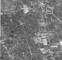
(a) raw data January 29, 1997
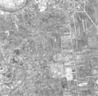
(b) geometric corrected December 10, 1995
Fig. 2 North of Bangkok OPS images
Fig. 3(a), shows corresponding window area cropped from uncorrected image. (Fig. 2 (a)) as Fig. 3(b) show the searching areas, where are spreadly selected through out the corrected image (Fig. 2 (b)) and cropped to be size of 32*32 pixel. Two sub images are used for typical experimentation.
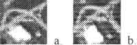
Fig. 3 Window area and search area
The second step is to apply the statistical correlation as mentioned before on a pair of sub scene to carry out the correction point, Rs(u,v) peak. Fig. 4 show, the searching areas, where are decorrelated by whitening filter (G) with p = 0, 0.5, 0.9 and 1, respectively.
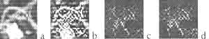
Fig. 4 Decorrelated search area p = 0, 0.5, 0.9 and 1 respectively
Fig. 5 shows the Simulation results of correlation measure with p=0, 0.5, 0.9 and 1. It is obviously shown that clearly show the two last results have the highest peak of correlation and easier to point out. By using the same procedure, the other 7 points are performed referring as ground control points (GCPs) and user for geometric transformation with bilinear technique (Eq. 20 and 21). They6 gray level interpolation have been performed with bilinear interpolation (Eq. 22) in last step and the final result of geometric correction has been shown in fig 6.
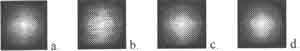
Fig 5. Simulation results of Static correlation measurement with p=0, 0.5, 0.9 and 1
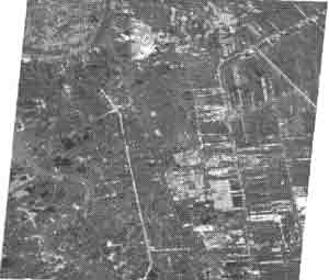
Fig 6. Final result of geometric correction image.
5. Conclusion
The basic correlation has been developed for easily distinguish the peaks of Rs(u,v) with statistical correlation technique. The results show that Rs(u,v) peaks sharply at the correct pointand caan be the reliable automatically geometric based on image to image registration.
References
- W. F. Webber, "Techniques for Image Registration," IEEE Con. On Machine Processing Remotely Sensed Data. Pp. 1B.1-1B.7, Oct. 16-17, 1973.
- W. K. Pratt, "Correlation Techniques of Image Registration," IEEE Trans Aerosp. Electron. Syst., Vol AES-10, pp. 353-258, May 1974.
- A. Arcess, P. H. Mengert, and E. W. Trombini, "Image Detection through Bipolar Correlation," IEEE Trans. Information Theory, Vol. IT-16, pp. 534-541, Sep. 1970.
- R. C. Gonzalez and R. E. Woods, Digital Image Processing, Addition-Westery Publishing Company, USA, Sep. 1993.
- W. K. Pratt, "Generalized Wiener Filtering Consumption Techniques," IEEE Trans. Computer, Vol. C-21, pp. 636-641, July 1972.