| GISdevelopment.net ---> AARS ---> ACRS 1998 ---> Poster Session 2 |
Identification of Damaged
areas Due to the 1995 Hyogoken-Nanbu Earthquake Using Satellite Optical
Images
Masashi Matsuoka and Fumio
Yamazaki
Earthquake Disaster Mitigation Research Center, RIKEN
2465-1 Mikiyama, Miki, Hyogo 673-0433, Japan.
Tel: (81)-794-83-6632 , Fax : (81)-794-83-6695
E-mail : mastuoka@miki.riken.go.jp
AbstractEarthquake Disaster Mitigation Research Center, RIKEN
2465-1 Mikiyama, Miki, Hyogo 673-0433, Japan.
Tel: (81)-794-83-6632 , Fax : (81)-794-83-6695
E-mail : mastuoka@miki.riken.go.jp
Several earth observation satellites observed the Kobe area before and after the 1995 Hyogoken-Nambu, Japan Earthquake. Since a part of the damage survey results of this earthquake is maintained as GIS data, a quantitative analysis of the surface change in damage areas is possible. Spectral characteristics of the area damaged by the earthquake were investigated using LANDSAT and SPOT satellite optical images taken before and after the earthquake for examination the possibility of extracting the earthquake damaged distribution by satellite remote sensing. The damage distribution extract by discriminant analysis of the spectral characteristics agreed with the results of an actual damaged survey.
Introduction
Satellite remote sensing, which easily monitors a large area, could provide effective information at the time of recovery activity, e.g., forming a restoration plan, if it is able to know the distribution of the damage due to disasters at an early stage. Several satellites observed the Kobe area before and after the 1995 HYOGOKEN_Nanbu Earthquake (Sudo et al., 1995). Multispectral characteristics were different between images of the liquefied areas and burned areas taken by airborne remote sensing just after the earthquake occurred (Mitomi and Takeuchi, 1995). A study suggested the possibility of interpreting the damaged area based on the spectral pattern changes between satellite image taken before and after the earthquake (Inanaga et al., 1995; Yoshie and Tsu, 1995). However, no quantitative approach was found for examining the possibility of identifying the damage distribution from the relationship between the spectrum characteristics of the damaged area by satellite images and detailed survey results.
Since part of the damaged survey results of this earthquake was maintained as GIS data, a quantitative analysis of the surface in the damaged area is possible. In this study, the spectral characteristics of the damaged due to this earthquake were investigated using LANDSAT and SPOT satellite image taken before and after the earthquake. Then the relationships between damaged distribution extracted through discriminant analysis of satellite images and survey data were evaluated.
Data
Earthquake Damage Survey Data: Liquefaction and building damage were focused on as earthquake damaged in this study. Boiled sand deposits due to the earthquake are digitized on the 1/50,000 scale ground failure survey map (Hamada et al., 1995) and used as liquefied area data. The building damaged data based on detailed survey results compiled by AIJ (the Architectural Institute of Japan) and CPIJ (the City Planning Institute of Japan), and digitized by BRI (Building Research Institute, Ministry of Construction) were utilized as GIS data. In the GIS data, the building damage level was classified into the five categories: damage by fire, severe structural damage, moderate damage, slight damage and no damage, and the numbers of damaged building were totaled for each block in cities (Building Research Institute, 1996).
Satellite Image: The SPOOT/HRV and LANDSAT/TM observed the area of interest on January 20, and January 24, 1995, respectively. We used the images taken on March 22, 1990 by SPOT and on August 17,1994 by LANDSAT for data before the earthquake, and aimed to examine the change in spectrum characteristics for the damaged area. The region of the satellite images is shown in Fig.1.
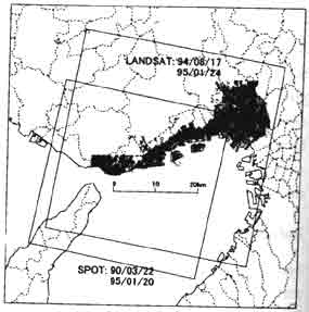
Figure.1 : Area of this study
Correction of Images: Because the digitized values in the satellite images were different depending on the observation situation and the surface conditions, the digital number (DN) correction was required before starting this study. First of all, clouds and cloud shadows covering the area were removed by using proper threshold values of several spectral bands. Areas of vegetation were also excluded from The images using NDVI (Normalized Difference Vegetation Index) because the reflection characteristics of the leaves of plants differ seasonally.
For DN correction, we selected pixels in nonliquefied and nondamaged areas from these images, using the liquefaction data and building damage data. Here, the selected pixels were considered to be the areas in which there was no change of the surface after the earthquake. Furthermore, the DN in the images taken before the earthquake for all areas were corrected so that the histogram of the selected pixel DN in this image fits that in the image taken after the earthquake.
Characteristics of the DN in the Earthquake-Damaged Area
The pixels that represent the area of liquefaction, burning, heavy damaged, slightly damage and no damage were selected from the images to examine the characteristics of the DN in the earthquake-damage area. The liquefied class contained pixels included in the liquefaction data. The pixels for the burned class were selected from the city blocks where all buildings were determined to have the severe or moderate structural damage and slightly damage, and categorized into heavy and slightly damage classes, respectively.
The pixels used for DN correction were those in the nondamaged class of damaged class. The 300 and 500 pixels for each class of damage were taken to analyze from the LANDSAT images and the SPOT images, respectively.
Relationship between LANDSAT Images and Earthquake Damage: The characteristics of the DN in each classified damage area due to the earthquake are shown in Fig.2. The mean value of the DN and the standard deviation in the damage classes are shown in Table 1. The DN are larger for all bands, other than band 6, in the liquefied area in comparison with the nondamaged area. The DN of the burned area is smaller than that of the nondamaged area, but the DN of the heavy damaged area is similar to that of the nondamaged area. The mean value of the DN and the standard deviation in the damage classes before the earthquake are shown in Table 2,and the difference in the DN in classified damage area before and after the earthquake are shown in Fig. 3 and Table 3. like the liquefied area, the DN is high for all bands other than band 6. for the burned area, the DN in the blue light range of band 2 was especially low.
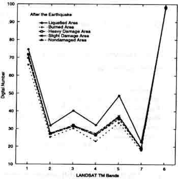
Figure.2 : Spectral features of LANDSAT/TM bands for damaged area after the earthquake.
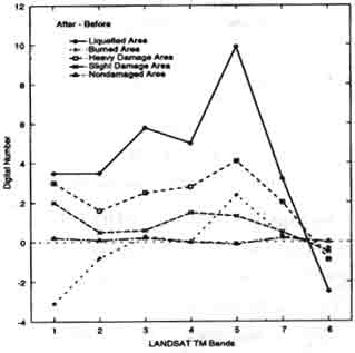
Figure.3: Change in digital numbers of LANDSAT/TM bands for damaged areas before and after the earthquake
These results are in good agreement with the damage survey performed by airborne multispectral scanner remote sensing (Mitomi and Takeuchi, 1995). The DN in the heavy liquefied area, did not greatly differ from the values in the nondamaged area. However, the DN of band 1 in the blue light range was a somewhat high in comparison with the nondamaged area.
The DN in the liquefied area was high in the range from the visible to mid-infrared bands, because of the higher reflectance of sand than the surface of asphalt. Also, it is conceivable that the DN was raised in infrared bands in the heavy damage due to the exposure of soil under mud walls and roofing tiles upon the collapse of old wooden dwelling. The increase of reflection in the blue light band region is due to the roofs of the building being covered with the blue vinyl canvas sheets in the building damage areas.
| Classified damaged area | Number of pixels | Digital number: Average (sd.) | ||||||
| 1 | 2 | 3 | 4 | 5 | 6 | 7 | ||
| Liquefied | 300 | 74.5(6.6) | 31.9(4.5) | 40.3(7.6) | 32.2(6.5) | 48.9(12.4) | 97.6(2.0) | 22.7(6.6) |
| Burned | 300 | 66.0(3.9) | 25.3(2.5) | 30.2(4.0) | 23.1(3.7) |
33.6(6.1) |
98.9(1.0) | 17.8(3.5) |
| Heavy Damage | 300 | 71.8(5.9) | 27.5(3.1) | 32.1(4.8) | 26.4(4.6) | 35.7(9.7) | 98.1(1.5) | 18.8(8.7) |
| Slight Damage | 300 | 71.6(6.6) | 27.5(3.8) | 31.9(6.2) | 27.3(5.8) | 37.4(9.5) | 98.2(1.7) | 19.2(5.5) |
| No Damage | 300 | 69.8(5.6) | 27.0(3.6) | 31.4(5.9) | 26.5(5.6) | 36.8(9.7) | 98.5(1.9) | 19.1(5.6) |
| Classified damaged area | Number of pixels | Digital number: Average (sd.) | ||||||
| 1 | 2 | 3 | 4 | 5 | 6 | 7 | ||
| Liquefied | 300 | 71.0(6.8) | 28.5(5.4) | 34.5(9.2) | 27.2(8.3) | 39.0(15.5) | 100.0(1.7) | 19.5(6.6) |
| Burned | 300 | 69.1(4.0) | 26.1(2.5) | 29.9(3.9) | 23.1(3.5) | 31.2(5.7) | 99.2(0.5) | 17.5(3.1) |
| Heavy Damage | 300 | 68.6(4.9) | 25.9(3.0) | 29.5(4.9) | 23.6(4.6) | 31.6(7.2) | 99.0(0.9) | 16.7(4.2) |
| Slight Damage | 300 | 69.96(5.0) | 26.9(3.4) | 31.3(5.8) | 25.8(5.8) | 36.1(9.9) | 98.7(1.4) | 18.7(5.4) |
| No Damage | 300 | 69.6(5.0) | 26.9(3.2) | 31.3(5.3) | 26.5(5.2) | 36.9(8.8) | 98.5(1.8) | 19.1(5.0) |
| Classified damaged area | Number of pixels | Digital number: Average (sd.) | ||||||
| 1 | 2 | 3 | 4 | 5 | 6 | 7 | ||
| Liquefied | 300 | 3.5(7.6) | 3.5(5.4) | 5.8(9.0) | 5.0(8.3) | 9.9(14.5) | -2.5(2.2) | 3.2(7.7) |
| Burned | 300 | -3.1(4.2) | -0.8(2.3) | 0.3(3.8) | 0.0(3.3) | 2.4(5.2) | -0.3(1.1) | 0.3(3.5) |
| Heavy Damage | 300 | 3.0(4.9) | 1.6(2.8) | 2.5(4.5) | 2.8(4.4) | 4.1(9.2) | -0.9(1.4) | 2.0(8.6) |
| Slight Damage | 300 | 2.0(6.3) | 0.5(3.4) | 0.6(5.1) | 1.5(5.1) | 1.3(8.5) | -0.5(2.1) | 0.5(5.1) |
| No Damage | 300 | 0.2(5.8) | 0.1(3.4) | 0.2(5.3) | 0.0(5.0) | -0.1(8.7) | 0.0(2.3) | 0.2(5.2) |
Relationship between SPOT Images and Earthquake Damage: The DN after the earthquake and the DN difference before and after the earthquake in the classified damage areas are shown in Table 4 and Table 5, respectively, for SPOT images. The changes of the DN in earthquake damaged areas showed the same pattern as that in the LANDSAT images; the DN became high in the liquefied area. However the change of the DN in the burned or building damage area did not show such great difference compared with the nondamaged area. This coincides with results of previous research (Hosokawa and Zama, 1998). Because the sensor mechanism in LANDSAT is different from that in SPOT, there is the possibility that the sensitivities of the two sensors differ. Detailed examination will be necessary for further study.
Extraction of Damage Distribution Using LANDSAT Images
We tried to extract the earthquake damage distribution from the DN changes using the LANDSAT images, because the LANDSAT images were characteristics of spectral patterns before and after the earthquake.
Damage distribution was extracted by discriminant analysis using the DN after the earthquake and the difference in DN before and after the earthquake as the representative variables. The minimum distance classification method was used as the discriminant analysis. The discriminant table is shown in table 6. the liquefied or burned area was had a comparatively high coincidence ratio. The distribution of the heavy damage area (black part in Fig. 4) was in relatively good agreement with that of the actual damage survey result (Fig. 5), but the coincidence ratio of the building damage area was not very high.
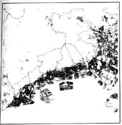
Figure.4 : Damage distribution estimated from TM images
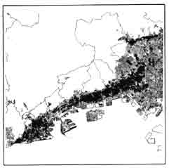
Figure.5 : Distribution of hard-hit areas based on building damage data by BRI
| Classified damaged area | Number of pixels | Digital number : Average (sd.) | ||
| 1 | 2 | 3 | ||
| Liquefied | 500 | 57.5(5.8) | 46.9(7.6) | 40.3(7.7) |
| Burned | 500 | 49.6(2.8) | 36.2(2.6) | 30.4(2.8) |
| Heavy Damage | 500 | 51.0(3.5) | 37.5(3.1) | 31.9(3.3) |
| Slight Damage | 500 | 51.1(3.7) | 36.9(3.2) | 31.2(3.3) |
| No Damage | 500 | 49.5(3.2) | 36.2(2.8) | 31.8(2.9) |
| Classified damaged area | Number of pixels | Digital number : Average (sd.) | ||
| 1 | 2 | 3 | ||
| Liquefied | 500 | 3.0(9.1) | 5.7(10.3) | 6.1(10.2) |
| Burned | 500 | -0.9(3.6) | -0.8(3.0) | -0.3(3.0) |
| Heavy Damage | 500 | 0.3(4.5) | 0.5(3.7) | 0.9(3.6) |
| Slight Damage | 500 | 0.9(4.7) | 0.1(3.7) | 042(3.5) |
| No Damage | 500 | 0.1(3.8) | 0.0(3.2) | 0.1(3.2) |
| Classified damaged area | Estimation from TM images | No. of pixels | Coincidence ratio (%) | |||||
| Liquefied | Burned | Heavy Dmg. | Slight Dmg. | No Dmg. | ||||
| Survey Result | Liquefied | 224 | 11 | 29 | 15 | 21 | 300 | 75 |
| Burned | 6 | 239 | 28 | 8 | 19 | 300 | 85 | |
| Heavy Damage | 14 | 42 | 144 | 51 | 49 | 300 | 48 | |
| Slight Damage | 20 | 27 | 78 | 108 | 67 | 300 | 36 | |
| No Damage | 17 | 36 | 53 | 46 | 148 | 300 | 49 | |
| No. of Pixels | 281 | 355 | 332 | 228 | 304 | 300 | 58 | |
Conclusions
We examined the spectral characteristics in area damaged by the 1995 Hyogoken Nanbu Earthquake, using LANDSAT/TM and SPOT/HRV images. The digital numbers of the liquefied area were high in the range of visible to infrared bands, whereas those of the burned area became low in the visible light range. The heavy damaged area shown a trend similar to the liquefied area. The extracted damaged distribution using the minimum distance classification agreed with damage survey results.
Acknowledgement.
We thank Prof. Saburoh Midorikawa of Tokyo Institute of Technology and Ms. Asako Inanaga of Remote Sensing Technology Center of Japan for their helpful advice. The LANDSAT and SPOT images used in this study were provided by Space Imaging EOSAT, SPOT IMAGE, and NASDA.
Reference
- Building Research Institute (1996). Final Report of Damage Survey of the 1995 Hyogoken-Nanbu Earthquake (in Japanese).
- Hamada, M., isoyama, R. and Wakamatsu, K.(1995). The 1995 Hyogoken-Nanbu (Kobe) Earthquake, Liquefied, Ground Displacement, and Soil Condition in Hanshin Area, Association for Development of earthquake Prediction.
- Hosokawa, M. and Zama, S. (1998). Comparison of Landcover Mapping Method Using Satellite Data for Extracting Area Damaged by 1995 Hyogoken-Nanbu Earthquake, Technical Report of National Research Institute of Fire and Disaster, No.85, pp.10-21 (in Japanese).
- Inanaga, A., Tanaka, S., takeuchi, S., Takasaki, K., and Suga, Y. (1995). Remote Sensing Data for Investigation of Earthquake Disaster, Proc. of the 21st Annual Conf. of the Remote Sensing Society, pp.1089-1096.
- Mitomi, Y. and Takeuchi, S. (1995). Analysis of spectral Feature of the Damaged Areas by liquefaction and Fire Using Airborne MSS Data, Proc. of the 18th Japanese Conf. on Remote Sensing, pp.117-118 (in Japanese).
- Sudo, N., Tada, t., Nakano, R., Cho, K., Shimoda, h., and Sakata, T. (1995). Multi Stage Remote Sensing on the Great Hanshin Earthquake Disaster Survey, proc. of the 18th Japanese Conf. on Remote Sensing, pp.115-116 (in Japanese).
- Yoshie, T. and Tsu, H. (195). Satellite Data Processing to Delineate the Densely Built-up Areas Damaged Disastrously By 1995 Hyogoken-Nanbu Earthquake, Proc. of the 18th Japanese Conf. on Remote Sensing, pp.119-122 (in Japanese).