A Linear-Feature Based Method for the Quality Assessment of Remotely Sensed Images

A Linear-Feature Based Method for the Quality Assessment of Remotely Sensed Images

Shue-chia Wang
Department of Surveying Engineering
National Road, Tainan, Taiwan
Fax: (+886)-6-2375764
E-mail: scwang@mail.ncku.edu.tw

Abstract
Judging the quality of remotely sensed imagery is very important. Especially when the decision has to be made whether an ordering image is of good quality and should be paid for. There are many ways to label the quality of a imagery, ranging from subjective judgment by human eyes to objective judgment by some quality indices like the SNR, the MTF etc. In this paper we propose a new method for judging the quality of remotely sensed images. The new method is based on the number and the strength of the linear features contained in the images. It is simple and is more proper for judging the image quality than other methods when the ability to differentiate different objects is of main interest.

Introduction
With the increasing commercialization of remote sensing from satellites and airplanes, one problem arise between the purchasers and the providers of remotely sensed imageries. That is, should one images be judges as good so that the purchaser should accept it or it is of poor quality so that the purchaser has the right to reject it and withhold the payment.?

The same problem exists since long time in the society of Photogrammetry. There, the quality is judged by spatial resolution of the photograph. The best way to determine the resolution of aerial photographs is to use ground resolution test target. When this target is photographed in the image, the MTF (Modular Transfer Function) of that image can be estimated, which gives clue to the resolution. Details about this procedure can be found in every Photogrammetric textbook.

But for the remote sensing, it is not practicable to construct resolution test target and to lay it on the ground. Because on one hand the area covered by a single remote sensing image is usually very large, 60kmx60km for a SPOT image for example, and the atmosphere condition might vary from one place to another. One single target an not tell very much abut the overall quality of the whole image. On the other hand, the ground resolution of most commercial remote sensing imagery from satellites airplanes is much lower than the resolution of a photograph. That means if we intend to use the ground resolution test target, that target must be very large, some tens to hundreds of meters in size, which is not practical.

One frequently used method for judging the quality of digital images the SNR (Signal Noise Ratio). It is particular popular among the sensor design colleagues. Because the SNR represents very precise the performance of the hardware. But for an already acquired image, it is very difficult to obtain a reliable estimation of the SNR. Because the estimation of the size of the noise is a very complex problem. Canny (1986) defines the noise as anything which does not belong to step-like edge and uses his edge detector to separate the noise component. Meer et al. (1990) proposed a very complicated procedure to estimate the noise component of a digital image. Basically they define the noise as the variation of pixel values in the homogeneous area. Because the complexity of this estimation problem, both methods have to make some assumptions which are not always true. For example, both methods assume that the noise must be Gaussian white and that a certain percentile of the pixel value variation comes from the noise, etc. One theoretically more sounder approach is to separate the un-correlated part (the noise) from the correlated part (the signal) by the least squares collocation. This method has been successfully used to separate the random measuring error (the noise) from the systematic film deformation(the signal) by Kraus et al. (1972). It can be easily transferred to estimate the un-correlated Gaussian white noise in the digital image.

Defining that the noise is random, un-correlated, additive and stationary, then eh sensed pixel value g is composed of the signal s (the radiometric energy from the object) and the noise n

g = s + n (1)
Under the assumption of stationary and random noise, s and n are un-correlated. Denoting s2 as the variance, we then have

s²_g = s²_s + s²_n (2)
From equation (2) we can see that if s²_n is negligible small, it is obvious that the strength of the signal s²_s can simply be approximated by the s²_g, which can be estimated by the sample variance of pixel values. In general the noise component s²_n must be estimated in order to get the estimation of the signal strength s²_s.

The difficulty of using the SNR or the signal strength for judging the image quality lies not only in he estimation itself but also in the definition of noise. For example, it an image is used to recognize different kinds of crops in the field based only on the spectral reflectance of each particular kind of crops, than the small gaps between each individual plant, which expose the back ground soil, would act as noises, since they will disturb the recognition and preferably should be filtered out. But these gaps actually reflect the true situation and are signal in physical is used to count individual plants, than the gaps between the plans are important signal, because they provide the information for the necessary differentiation between each individual plant. This simplified and not very realistic example is only trying to point out that we define in the object recognition as signal and noise might not be the same as those defined purely from the physical point of view. In digital image processing this phenomenon is called the scale of space.

Despite whether the noise is negligible or not, the main usage of remote sensing images is to recognize objects on the earth surface. In order to recognize objects, the image must be able to differentiate between different objects i.e. there must be enough differences in pixel values between different objects. Pixel value differences is called gradient in the digital image processing and can be detected by edge detector techniques. From this point of view, the quality of a remotely sensed images can also be judged by the richness of the edges in it.

The major advantage of judging the image quality by edge is that we can easily avoid the problem of estimating the noise strength. We will see this later in more detail.

Quality Assessment through Estimation of Signal Strength
Although as mentioned in the previous chapter that judging the images quality by signal strength is very difficult, we will nevertheless demonstrate this method by some examples as comparison to our new method.

For a image of the size n x n, the overall variance of pixel values can be estimated by

(3)

where

is the estimated sample variance,
g is the pixel value of the ith line and jth sample

is the sample mean of all pixel values of the image

As started in Eq. (2), this overall variance is composed from two parts, the signal part and the noise part. In the absence of noise, the signal strength is equal to the overall variance. As already mentioned, the real problem of using this index for judging the image quality is in the presence of the noise. In that case, one should use a proper method to estimate the variance of the noise first, than use Eq. (2) to subtract the s2g to get the estimated variance of the signal s2s. Here again we would like to emphasize once more that a strict estimation of the noise strength is very difficult.

Fortunately, for out purpose of judging the image quality only relatively, the accuracy of the estimated noise strength does not play an important roll. Because on one hand, very noisy images need not to be judged. Everyone will agree that they are of poor quality. On the other hand, if the images are of good quality thus with very noise strength does not affect very much the estimation of the relatively strong signal strength.

A stereo pair of SPOT images with 1000x 1000 pixels of XS bands (2000x2000 pixels in Panchromatic) cover a mountain area in middle Taiwan are used to demonstrate the quality assessment using this method. Most part of the sensed area is covered by dense forest. Only along the river in the middle of the images there are some small flat areas with small villages and rice fields. The original images in panchromatic (B/W) and in three bands (G,R,IR) are shown in Fig. 1. Judged by bare eyes one can clearly see that for the small part along the river valley covers village and rice field, the left images numbered 299303L has better quality than the right image 299303L . Because the houses and rice fields appear more clearly. But when the large mountain area is concerned, the right image has superior quality. Because it shows more reason is that in the large mountain area. The reason is that in the left image there is a thin film of haze hanging over the mountain, which reduces the contrast. This labeling the image quality. If the image covers a very large area, it is sometimes impossible to use one single value to label it's quality.

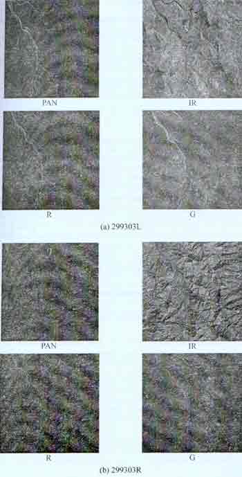
Fig. 1 Spot stereo oair in PAN and XS bands covering a mountain area in Taiwan
In order to label the image quality by the signal variance, we have to estimate the noise variance first. Since we know already that the noise is not strong in both images, no elaborated method like those previously mentioned is used to estimate the variance of the noise. Instead, we assume that in the most homogeneous areas, the signal is zero and that the pixel value variance is that noise variance itself. 20 most homogeneous areas of the size 5x5 pixels and 7 x 7 pixels are selected. Their variances are calculated and average. We simply take this average to be the estimated noise variance.

The overall variances and the nose variances for the original 299303L and 299303L are listed in the first two columns in Tab 1. We can see that for all three XS bands and the PAN band, none of the noise variances exceeds 2. The thin haze in the left images does not affect the estimation of noise strength. Comparing to the overall variances of the whole images, the noises are negligible for judging the quality of the image. Therefore in our examples, it is enough to judge the image quality by looking only to their overall variance. We would say that except for the green band. But we know that if only the river valley is concerned, the judgment should be reversed.

Tab.1 Variance estimation of the SPOT images

Image	299303L				299303R				299303L corrupted
Band	B/W	G	R	IR	B/W	G	R	IR	B/W	G	R	IR
Overall variance	131	143	70	421	96	48	92	482	181	191	120	470
Noise variance	0.2	0.3	0.8	1.9	0.0	0.0	0.1	0.1	45	40	43	45

We can also demonstrate the disaster of neglecting the noise strength when it is in fact not small. For this demonstration we purposely add Gaussian white noise with variance 72 to 299303L. The overall variance and the noise variance of these artificially corrupted images are listed in the third column of Tab 1. We can see that if we neglect the large nose variances of 299303L and simply use the overall variances for judging the image quality, we would get the wrong conclusion that 299303L is better than 299303R.

Quality Assessment by Linear Features
Linear features can be detected by the so called edge detectors. Since all edge detectors are more or less based on the computation of gradients (grey value differences between adjacent pixels), our quality assessment method by linear features is to some extend also related to the previous method based on the variance estimation. Because variance represents also the degree of variation in grey value, but more of global variation. While edge detectors looks only for local differences.

It is well known that gradient is very sensitive to noise, and we have seen from the previous demonstration dangerous the noise could be, therefore it might seem not to be a wise idea to use linear features for judging the quality. But by using a very small trick we can totally avoid the influence from noise. This is exactly the reason why we propose this method. We know that random noises are un-correlated and can not cause long linear features, therefore simply by limiting the minimum length of the linear features, we can get rid of the problem associated with noises. Also the problem of the definition of noises is also easily solved by choosing a proper size for the mask of the edge detectors. It is a common practice in the edge detectors. It is a common practice in the edge detecting to filter out or to suppress high frequency signals which would disturb the detection. For example, by selecting a proper size of the LoG or the Canny operator mentioned below, signals above a certain frequency can be smoothed out. Here we can use this ability to solve the problem according our purpose of application, information above a certain frequency should be treated as noise, then by choosing a proper size for the edge detector, all information higher then that frequency can be effectively suppressed.

There are many well known edge detector methods. Any one could be used for our purpose. Important is that after edge detection, the detected edge elements have to be linked together to form linear features. Since our goal is to compare image quality relatively, it makes no difference which edge detector and which edge linking method are used. As long as all the images are judged by the same methods, relative comparison of their quality unchanged.

In our experiment we use the Zero-Crossing method proposed by Marr et al. (1980) for detecting the edge elements. Since their original operator reacts also to very weak edges, we have set a proper threshold to suppress very weak edges. The linking is achieved by simply following the flagged pixels of zero-crossing. Two indices can be derived for judging the image quality. One is the total number of linear features in the image. The second is the average length of the linear features. The same two SPOT images as used in the previous chapter are used to demonstrate this new method.

Table 2. shows the quality assessment results. Similarly like Tab 1, image column 1 and 2 are for the original images and the third column is for the artificially corrupted 299303L. We can see that in the absence of noise. 299303R has more linear features than 299303L. According to our definition of image quality, 299303R is better than 299303L. Therefore the linear features method shows the same results as the variance method.

Tab. 2 Quality assessment by linear features for the SPOT images

image	299303L				299303R				299303L corrupted
Band	B/W	G	R	IR	B/W	G	R	IR	B/W	G	R	IR
#linear features	11995	6708	3104	3627	14068	7985	4371	3085	4613	2194	1384	1821
Average length	9.0	8.8	9.0	8.9	9.1	9.3	9.0	9.1	9.0	8.8	9.0	8.9

From the third column we can see that the linear features method still indicates that 299303R is of better quality than the corrupted 299303L. Our method is not affected by the artificially added noise . Remember that while using the variance method for judging the image quality, if the noised strength is not considered, the corrupted 299303L will be wrongly judged as better. Here again we see the advantage of linear feature based method. There is no need to do any elaborated estimation of the noise variance.

Conclusion
With increasing commercialization of satellite images, objective quality assessment of remotely sensed images becomes more important. Since the payment or the acceptance of ordered images depends on the image quality.

After analyzing the quality assessment method based on the estimation of the signal strength, we proposed a very simple linear-feature based method for assessment of the image quality. The new method is much easier to implement because it does not have to do the very complex estimation of the noises. The computation is much less than the traditional variance method. The only weakness of this method is that it gives no absolute measurement of the image quality. The index is only relative. Which means one need a "good" image as reference first and compare other images to this one to get the assessment of their quality. But for the practice, it is not a problem to select a proper reference image.

References

Canny, J. 1986 "A computation approach to edge detection." IEEE Trans. PAMI, vol. 8, pp. 679-697.
Kraus, K.; Mihail, E. M. 1972: "Linear Least-Squares Interpolation." Photogrammetric Engineering. Vol. 38, pp. 1016-1029.
Marr, D.; Hildreth, E. 1980: "Theory of Edge Detection." Proceedings Royal Society London., Vol. B207. pp. 187-217.
Meer, P.; Jolion, J. M.; Rosenfeld, A. 1990: " A Fast Parallel Algorithm for Blind Estimation of Noise Variance." IEEE Trans. PAMI, Vol. 12. pp. 216-223.