| GISdevelopment.net ---> AARS ---> ACRS 1998 ---> Poster Session 1 |
A Study of Neural Network
Classification of Jers-1/Ops Images
Yuttapong Rangsaneri, Punya
Thitimajshima, and Somying Promcharoen
Department of Telecommunications Engineering,
Faculty of Engineering
King Mongkut's Institute of Technoloyg
Ladkrabang, Bangkok 10520, Thailand
E-mail: kryuttha@kmitl.ac.th, ktpunya@kmitl.ac.th
Abstract
Department of Telecommunications Engineering,
Faculty of Engineering
King Mongkut's Institute of Technoloyg
Ladkrabang, Bangkok 10520, Thailand
E-mail: kryuttha@kmitl.ac.th, ktpunya@kmitl.ac.th
In this paper, the multiplayer perceptron (MLP) neural network using the back-propagation (BP) algorithm is studies for the classification of multispectral images. The network architecture is made up of three layers: the input layer, one hidden layer and the output layer. The number of input nodes is specified by the dimension of the image to be categories. A simulation has been made and the experimental results on JERS-1/OPS image are given in comparison with the Gaussian maximum likelihood classifer.
1.Introduction
The maximum likelihood algorihm based on Gaussian probability distribution functions is considered to be the best classifier in the sense of obtaining optimal classification rate. However, the application of neural network to the classification of satellite image is increasingly emerging. Without any assumption about the probabilistic model to be made, the networks are capable of forming highly non-linear decision boundaries in the feature space and therefore they have the potential of outperforming a parametric Bayes classifier when the feature statistics deviate significantly from the assumed Gaussian statistics.
In this paper one of neural network, the multiplayer perceptron (MLP) model using the back-propagation (BP) algorithm, will be studies to classification the four categories of Japanese Earth Resource Satellite/Optical Sensore (JERS-1/OPS) . The fundamental of this kind of neural network is described in first section. In the second section, the data of JERS-1/OPS is discussed, and we describe about the network and parameter selection in the following section. Finally, the classification result are given and compared to those obtained by the Gaussian maximum likelihood classification.
2 MLP model and BP algorithm
The multiplayer perceptron (MLP) model using the back-propagation (BP) algorithm is one of the well-known neural network classifiers which consist of sets of nodes arranged in multiple layers with connections only between node in the adjacent layers by weights. The layer where the inputs information are presented is known as the input layer. The layer where the processed information is retrieved is called the output layer. All layers between the input and output layers are known hidden layers. A schematic of a layers MLP model is shown in Fig. 1.
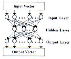
Fig 1. Schematic of a 3-layer MLP model.
For all nodes in the network , except the input layer nodes, the total input of each node is the sum of weighted outputs of the nodes in the previous layer. Each node is activated with the input to the node and the activation function of the node [1]. In Fig 2, node computations is shown.
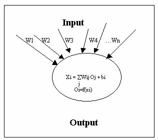
Fig 2. Node computations
The input and output of the node I (except for the input layer) in a MLP mode, according to the BP algorithm [1] [2], is :
Output: Oi = f(Xi) (2)
Where
Wij : the weight of the connection from node I to node j
Bi : the numerical value called bias
F : the activation function
The sum in eq. (1) is over all nodes J in the previous layer. The output function is a nonlinear function which allows a network to solve problems that a linear network cannot solve [3]. In this study the Sigmoid function given in eq. (3) is used to determine the output state.
Back-propagation (BP) learning algorithm is designed to reduce an error between the actual output and the desired output of the network in a gradient descent manner. The summed squared error (SSE) is defined as:
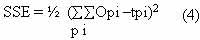
Where p index the all training patterns and i indexes the output nodes of the network. Opi and Tpi denote the actual output and the desired output of node, respectively when the input vector p is applied to the network.
A set of representative input and output patterns is selected to train the network. The connection weight Wij are adjusted when each input pattern is presented. All the patterns are repeatedly presented to the network until the SSE function is minimized and the network "learns" the input patterns. Applications of the gradient descent method [3] yields the following iterative weight update rule :
Where
D: the learning factor
a: the momentum factor
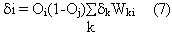
di: the node error, for output node I is then given as
The node error at an arbitrary hidden node is
For details BP algorithm including derivation of the equation see[1][2].
3 JERS-1/OPS image data
The JERS-1/OPS (Japanese Earth Resource Satellite / Optical Sensors) image data which used to training and testing the classification of the neural network is the area of Chantaburi city, Thailand. This image data consists of three bands: band 1 (0.52-0.60 mm), band 2 (.63-0.69 mm) and band 3 (0.76-0.86mm), and was taken on December 12, 1996. the image size is 256 x 256 pixels. Band 2 of this image is shown in fig. 3.
The aim of the classification with the neural network was to distinguish between the four categories : water, urban, vegetation and bare soil. The result was to be compared with the Gaussian maximum likelihood classification.
Two small sets of pixels were chosen to be the training and the testing sets of both methods (the neural method and the maximum likelihood method) are shown in Table 1.
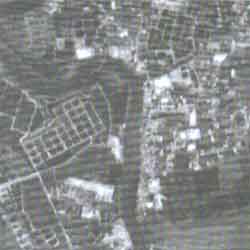
Fig.3. Band 2 of JERS-1/OPS image.
| Category | Train pixels | Test pixels |
| 1. Water | 217 | 1,023 |
| 2. Urban | 104 | 487 |
| 3. Vegetation | 135 | 469 |
| 4. Bare Soil | 92 | 255 |
| Total | 548 | 2,334 |
4 Network and parameter selection
We select three-layer MLP model using the back-propagation (BP) algorithm in this study. The number of input nodes is specified by the dimension of the input patterns. For the JERS-1/OPS image data, the input pattern is from one pixel consists of three bands at a precision of 8-b/band to give 24-b per input pattern.
Similarly, the output nodes are determined by the number of categories to be classified or the desired output mapping. In this paper, we classify four categories. Therefore, we have four bits per output pattern. Each bit of the desired output Tpi in eq. (4) presents state 1 or state 0, state 1 for "belongs to" and state 0 for "not belongs to" a category (eg., 1 0 0 0 is the desired output pattern for "belongs to" category 1).
The number of hidden nodes usually define at least as number of nodes in the input layer [5]. Based on Kolmogorov theory [6], 2N+1 hidden nodes should be used for one hidden layer (where N is number of input nodes). For 24 input nodes, we will have 49 hidden nodes. The learning factor (h) and the momentum factor (a) in eq. (5) are set to 0.01 and 0.9, respectively. The summed squared error (SSE) in eq. (4) is set to 0.003. In tble 1, the number of pixels in each category which we selected to train the neural network is shown.
5 Result
We designed MATLAB program to train this network on Pentium pro 200 workstation (64 MG RAM), and used 2 " days for training time. After training process, 2,334 pixels in table 1 was selected to test the correct classification percent of two methods (the neural network method and the maximum likelihood method (The results are shown in Table 3 and Table 4, respectively.
As is possible to see by reading the table, the neural network method seem to work a little better, The overall correct classification for the neural network method is about 92.8 percent, and the 85.6 percent value for the maximum likelihood method. This situation is explained by a better attribution in the neural network case of water, urban and vegetation categories, whereas the maximum likelihood method make less errors than the neural network method in one case which is bare soil category.
| True Category | Clasified as | Correct (%) | |||
| Water | Urban | Vegetation | Bare Soil | ||
| Water | 953 | 4 | 8 | 58 | 95.5 |
| Urban | 22 | 465 | 0 | 0 | 98.9 |
| Vegetation | 5 | 0 | 563 | 1 | 72.2 |
| Bare Soil | 63 | 0 | 8 | 184 | 72.8 |
| Overall accuracy | 92.8 | ||||
| True Category | Clasified as | Correct (%) | |||
| Water | Urban | Vegetation | Bare Soil | ||
| WAter | 908 | 0 | 21 | 94 | 88.8 |
| Urban | 0 | 395 | 0 | 92 | 81.1 |
| Vegetation | 0 | 0 | 443 | 126 | 77.9 |
| Bare Soil | 0 | 0 | 3 | 252 | 98.8 |
| Overall accuracy | 85.6 | ||||
6 Conclusion
The MLP neural network model using the BP algorithm for classification of JERS-1/OPS image data was simulated and processed. We found that, it is easily modified to accommodate more channels or to include spatial and temporal information. The input layer of the network can simply be expanded to accept the additional data. Although it is slow to train, but it is fast in the classification state.
Acknowledgement
The authors with to thank the National Research Council of Thailand (NRCT) for providing the satellite image data.
Reference
- J.L. McCelland and D. E. Rumelhar, Eds., Parallel Distributed Processing, Vol. 1. Cambridge, MA : MIT Press, 1986.
- Y.H. Pao, Adaptive pattern Recognition and Neural Network, Addition-Wesley Publishing Company, Inc., 1989.
- J.A. Bendiktsson, P.H. Swain and O.K. Ersoy, "Neural Network Approaches Versus Statistical Methods on Classification of Multisource Remote Sensing Data", IEEE Trans. Geosci. Remote Sensing, vol. 28, pp. 540-552, July 1990.
- H. Bichof, W. Schneider and A.J. Pinz, "Multishpectral Classification of Landsat Image using Neural Networks", IEEE Trans. Geosci. Remote Sensing. Vol. 30, pp. 482-480, May 1992.
- P.D. Heermann and N.Khozenie, "Classification of Multispectral Remote Sensing Data Using a Back-propagation Neural Network", IEEE Trans. Geosci, Remote Sensing, vol. 30, pp. 81-88; Jan. 1992.
- A.J. Annema, Feed-Forward Neural Network : Vector Decomposition Analysis Modeling and Analog Implementation, Kluwer Academic Publishers , 1995.