| GISdevelopment.net ---> AARS ---> ACRS 1998 ---> Agriculture/Soil |
Modeling Spatial Crop
Production: A GIS Approach
Satya Priya, Ryosuke
Shibasaki and Shiro Ochi
Center for Spatial Information Science, University of Tokyo
7-22-1, Roppongi, Minato-ku, Tokyo 106, Japan
Fax: 81-3-3479-2762
E-mail: satya@skl.iis.u-tokyo.ac.jp
Abstract:Center for Spatial Information Science, University of Tokyo
7-22-1, Roppongi, Minato-ku, Tokyo 106, Japan
Fax: 81-3-3479-2762
E-mail: satya@skl.iis.u-tokyo.ac.jp
Spatial Erosion Productivity Impact Calculator (Spatial-EPIC) gave a new direction to simulate crop production at regional scale based on microscopic simulation at each small piece of land in an efficient way. The result presented in this paper is based on existing/available spatial agro-climatic dataset but information related to soil and water has not been included spatially at this stage as they are under process of development. Using Spatial-EPIC crop model observed crop yield for the period 1995-1993 are compared with yields simulated and it is found that agreement between simulated and observed crop yield shows better correlation.
Introduction
GIS based modeling of an agroecosystem is expected to give a new approach in order to provide agricultural managers with a powerful tool to assess simultaneously the effect of farm practices to crop practices to crop production in addition to soil and water resources. At present, most of the crop models are location explicit information. Therefore, development of spatially or raster based biophysical crop model with go a long way in helping us to understand many intricacies of modeling of large areas at 1 to 10 km resolution. The large-scale distribution of crops is larges determined by climate. This study gives a preliminary result of Spatial-EPIC (which is in the process in identifying weakness of GIS data interpolation capabilities. We focused our efforts mostly on climatic dataset generation for three major crops Maize-Wheat-Rice which can be further used to analyze the response of other natural systems to climate change in a later course. The scale resolution of most crop models used in simulating climate change impacts is, for all practical purposes, a single point on the earth's surface. To get regional estimates of crop responses to climate change requires either scaling up the model simulations from point estimates or scaling up the data inputs from point measurements and then performing the simulations. Both ways will result in some loss of information due to aggregation error. The effect of spatial scale of climate inputs on crop simulation is examined in this study.
The purpose of this paper is to examine the effect of spatial aggregation (i.e, the size of the areas from which the synthesis of multiple in situ data points into a single areal estimate is made) of climate data used in crop models and find an agreement between modeled and observed crop yields. We begin with interpolation of WMO data at the degree (almost 10km on ground) grid resolution. Specifically this paper evaluates the relative impacts of climate and crop spatially throughout the study area.
Materials and Methods
In this section, the followings are described; the region of the study, 1) the crop model used in the analysis , 2) the modeling of climate data to a climate model grid network and 3) the procedures used to compare observed and simulated yields over a continuum of spatial scales within the grid network. The area chosen for this study compasses one of the northeastern state of India namely Bihar. The area studied is located between 21° 58' to 27° 31' North latitude and 83° 19' to 88° 17' East longitude. It is overlain at 10km grid size, which cover the entire state Bihar (Figure 1). Three different crops were modeled for the period of 1985-1993 using (Spatial-EPIC) a crop growth model described below. In northern India there are two distinct seasons Kharif (July to October), and Rabi (October to March). Therefore the crops modeled were Kharif maize, Rabi wheat and kharif rice at every two year crop rotation. The period between March to June (locally called as Zaid season) left fallow during the simulation. This distribution mimics the predominant crops, which is being taken widely in the area.
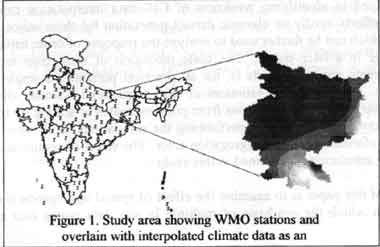
Figure 1. Study area showing WMO stations and overlain with interpolated climate data as an
Simulation Models:
Until now there have been a lot of studies on agricultural potential productivity but to relate actual crop productivity, model based simulations are not adequate. Estimates of on-farm and off-farm productivity are being done using experimental/point based model. Biophysical spatial based model is still lacking to compute them at regional or national level. Simulation models, such as EPIC (Willimas, 1990) model used was originally point-based developed by USDA-ARS. The first results of Spatial-EPIC being developed by the author is presented in paper (described below) together with mathematical presentation of the biophysical crop simulation process. The model is designed to predict what would happen under different conditions, such as change in temperature, precipitation, atmospheric CO2, soil moisture and so on at regional/national scale. The results presented in this paper are based on climate data. A model developed by Richardson (1981) was selected for use in EPIC because it simulates temperature and radiation, which are mutually correlated with rainfall. The weather generator module offers a convenient method of obtaining the numerous long sequence weather data that are required for the simulat
Spatial-EPIC
Spatial-SPIC is a crop simulation model being developed to estimate the relationship between soil erosion and crop productivity, which has been implemented in GIS environment to have spatial distribution of crop output. In addition to the plant growth routine, the model includes components for weather simulation, hydrology and crop management. It operates on a daily time-step. Among factors simulated by EPIC are evapotranspiration (based on Penmen Monetih model), soil temperature, crop potential growth, constraints and yields. EPIC uses a ssingle model for simulating all crops, although, of course, each crop has unique values for model parameters. For this study, CO2 concentration held at current ambient level (350ppm) has been used. Crop yields are estimated by multiplying the aboveground biomass at maturity (determined by accumulation of heat units of specific field harvest data) by a harvest index for the particular crop.
Preparation of spatial-EPIC Dataset
Model requires data on soil properties, which has been assumed same for all the area as Spatial-EPIC is under progress and data required for these parameters are under development. The detailed profiles of relevant production characteristics (for example, fertilization, planting, harvesting, irrigation and heat units for maturity) were complied for the crops simulated across the region. The range of values for those production characteristics is shown on table 1. the weather variables necessary for those production characteristics is shown on table 1. The weather variables necessary for driving the EPIC, a main impetus of this paper, are daily values of precipitation, minimum/maximum are temperature, solar radiation and humidity. A detailed discussion of climatic data generation is described in the next section.
| Maize | Planted | 7thJuly |
| Total Fertilizer(urea+elem.-Phosphorus) | 40+10 kg | |
| Total no. of irrigation/amount, (500/800) | 2/1300 mm | |
| Wheat | Sown | 10th November |
| Total ertilizer(urea+elem.-Phosphorus) | 75+15 kg | |
| Total no. of irrigation/amount, in 3 splits | 3/3000 mm | |
| RiceWithout Irrigation | Planted | 7th July |
| Total Fertilizer (urea+elem.-Phosphorus) | 40 +10 mg |
Data Generation: interpolation and interpretatio
Most simulation model assumes homogeneous conditions over the space they are representing. In general, these conditions do not exceed a few square kilometers in extent. To input weather data across India, for example, we were faced with the problem of extending required model input over several hundred square kilometers between weather stations. Several interpolation procedures are available, ranging from simple linear interpolation techniques and triangulated networks, to more sophisticated distance weighing or kriging techniques. It must be remembered that the only information used by any interpolation procedure is the location of known values. For this study, the climatic information used to make interpolation is based on inverse distance weighted method of more than 200 stations in India from which Bihar has been delineated for the purpose. While interpolation of a value at reach cell in the study area using 200 meteorological stations is technically easy, but some important questions can be raised : are the stations representative of the areas around them? How large or small an area do they represent? How does the spatial feature in question change over space? Is it continuos or discontinuous and abrupt?
We used same climate dataset for the different maps resolution across study area. Depending on its cell size, the level of detail becomes available at different resolution. It is thus important to realize the size of the dataset used to create GIS maps (as model input) and is important for model application from its accuracy and better performance view point. On the other hand a total of one or two stations falling in each administrative boundary may not be enough to give great confidence in the resulting interpolated map.
Results
Climatic data at 10 km spatial aggregation needs to be evaluated to identify its applicability in crop modeling; result of those are presented here. Observed yields were compared against simulated yields for two different grid cells of these there crops in the study area. As a mapping tools, GIS has been used for the production of descriptive maps using simulation model outputs that portray the spatial distribution of model prediction and the spatial juxtaposition of specified subsets of the data. The geographical locations of the modeled process of different crops are simulated actual yield but there is a lack on observed data to tie the results to a real world location. Figure 2 shows an example of comparing spatially distributed simulated crop yield with observed aggregated crop yield at district levels. The above results suggest that the aggregation of climate data alone showed pertinent agreement between observed and simulated yield, as the other parameters except climate remain unchanged. Observed data available for validation are average of district administrative boundary, whereas simulated output varies cell by cell as of their resolution. To check its validity more explicitly we averaged the simulated yield at district level as zonal mean productivity and then compared with observed average. Figure 3 shows a sample of linear regression between observed vs simulated crop yield of rice, wheat and maize in the year 86, 89 and 91 respectively. The outputs obtained on climate data gave quite satisfactory result and its is supposed that after introduction soil, topography and other input parameters spatially the model will yield a better result.
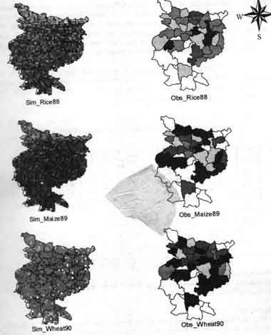
Figure 2. Comparing Spatially Distributed Simulated Crop Yield vs Aggregated Observed Crop Yield
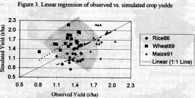
Figure 3. Linear regression of observed vs. simulated crop yields
Therefore, result reinforces the conclusion that in the range of spatial output examined here, agreement between observed maize, wheat and reice with simulated Spatial-EPIC model is sensitive and it depends a lot on the climate data.
Conslusion
Analytic operation allow GIS to generate new data correlation and prediction of future conditions. Research is still being conducted and preliminary results from this study are just becoming available. However, it is encouraging to have found a methodology that Provides a plant physiologist, a modeler and a GIS users a common ground to discuss simulation results and further potential research directions. Simulated crop yield maps generated can be used to better communicate model predictions. Hence using this methodology a region/nation can be modeled for crop productivity, which help researchers and decision-makers understand the status and extent of climate effects on global processes such as rice, wheat and maize production.
As of now, the most difficult problem countered in applying Spatial-EPIC areas in the developing world is the apparent lack of quality environmental data availability, detail validity, comprehensiveness, and scale must be carefully considered before this methodology can be successfully implemented.
Acknowledgements
This research is funded by "Research for the future" under the program of Japan Society for Promotion of Science.
References
- Satya Priya and Shibasaki, Ryosuke (1998). Soil Erosion and Crop Production: A Modeling Approach. Proceeding of Global Environment Symposium organized by Japanese Society of Civil Engineers held on 2-4 July at Osaka, Japan, pp175-180.
- Satya Priya and Shibasaki, Ryosuke (1998). Assessing Impact of Increasing Carbon Dioxide with Climate Change on Crop Production. Proceeding of International Conference on Modeling Geographical and Environmental Systems with Geographical Information Systems (GIS) held on 22-25 June at Chinese University of Hongkong, pp 72-77.
- Easterling, E. et. al., (1998). Spatial Scales of Climate Information for simulating Wheat and Maize Productivity: the case of the Us Great Plains. Agricultural and Forest Meteorology Journal 90 (1998) pp 51-63.
- Williams, J.R., Jones, C.A., Dyke, P.T., (1990). The EPIC model. EPIC-Erosion/productivity Impact Calculator: 1. Model Documentation USDA-ARS.Tech. Bull. NO. 1768, 3-92.
- Richardson, C.W. (1981). Stochastic simulation of daily precipitation, temperature, and solar radiation. Water Resour. Res. 17(I): 81-92.