| GISdevelopment.net ---> AARS ---> ACRS 1998 ---> Agriculture/Soil |
Remote Sensing and (GIS)
applications in the Erosion studies at the Romero river Watershed
Cristy Crema
Perlado
Agricultural Land Management and Evaluation Division Bureau of Soils and Water Management ,
Elliptical Road , Cor . Visayas A venue Diliman 1104
Quezon city, Philippines
Tel:6329320424 Fax: 6329204318
E-mail: bswm@pworld.net.ph
Abstract Agricultural Land Management and Evaluation Division Bureau of Soils and Water Management ,
Elliptical Road , Cor . Visayas A venue Diliman 1104
Quezon city, Philippines
Tel:6329320424 Fax: 6329204318
E-mail: bswm@pworld.net.ph
The land cover map derived from the satellite imagery showed that the watershed is dominantly covered with coconut and grasses which occur on practically all land from types (lowland to mountains). Forest occurs mostly on the steep to mountainous areas while rice is concentrated on the plain . Based on the GIS - generated maps , the estimated soil loss due to erosion is about 5 to 10 tons per hectare per year . This volume of the soil loss when translated to depth of soil is equivalent to about 0.1to 1cm. Topsoil in ten years. It can be concluded that although the satellite imagery showed a dominant agricultural land use , a minimal soil loss is expected for the next ten years.
Introduction The Romero River Watershed in Siniloan , Laguna was selected as perspective of a team approach in soil resources research under the BSWM Soil Research and Development Center (SRDC) - Japan International Cooperation Agency (JICA) Technical Cooperation Phase II . Soil Productivity Capability Classification (SPCC), one of the project components of the technical cooperation, is concerned with the development of database, soil rating system and soil management recommendations.
Data and information- collected ware inputted as part of the training on GIS and remote Sensing studies at the National Institute of Agro- Environmental Sciences (NIAES), Tsukuba City, Japan for the period June 16-August 8, 1997 under the supervision of Dr. Toshiaki Imagawa. Using TNT Map and Image Processing System (TNT mips),four (4) thematic maps (topographic, land slope)and one (1)derived map (land cover based on the landsat imagery) were prepared at a scale 1:75,000.
The second (post- training ) phase of the project involved erosion estimation study in the same area as one of the components of watershed analysis using PC Area . Mr. Kenji Matsumori, conducted the transfer of technology . Using the outputs of the NIAES training as polygon data set inputs, additional derived maps of the project site ware produced: (1) slope length map ,(2) Estimated soil loss (tons/ha/yr)map , and , (3)Estimated erosion depth (cm/10years).
The study was conducted to achieve the following objectives:
- To generate the geospatial database applying the principles of geographic information system(GIS) and remote sensing. And
- To conduct watershed analysis specifically erosion estimation studies.
Digitization of the topographic, soil, slope , and land use maps.
The four (4) sheets of the topographic map at 1:50,000 scale that covered the whole watershed ware scanned using a full color TIFF image file format . The scanned images Are then imported into the GIS software (TNT mips ), georeferenced , and mosaic ked . The watershed boundary was delineated/ digitized. The image was converted from raster to vector data and edited . The watershed boundary was extracted from the image and saved for printing .
The soil, slop ,and land use map ware scanned and saved in TIFF image file format . The scanned image ware then imported into the GIS software , georeferenced , and mosaic ked . The soil slope, and land use maps ware digitized and saved as vector spatial data and edited. Vector element attributes ware assigned such as titles legend , and color assignment to each mapping unit, setting the orientation , map scale and coordinates using unit setting the orientation , map scale and coordinates using the map and poster layout functions of TNT mips . The map file saved for printing.
Interpretation of LANDSAT TM data
Land sat TM data taken on the April 2, 1993 courtesy of NIAES was used in the study . The image was imported from ERDS. The watershed boundary was first extracted from the satellite imagery and the resulting vector data (watershed boundary ) was converted into raster. The land cover analysis of the watershed was done using the supervised classification function of the TNT mips . Attributes ware assigned to the vector elements and the file was saved as vector data.
Erosion studies and soil productivity estimation as component of watershed analysis.
The Universal Soil Loss Equation (USLE) was applied for the estimation of the annual soil erosion loss.
A = R* K * LS * C
Where : A is the amount of soil erosion (t/ha/year)
R is the rainfall coefficient
LS is soil coefficient
C is the plant / land cover coefficient
The rainfall coefficient (R) was presumed from rainfall intensity in 1994 (1868mm.annual rainfall) . The results of the Laboratory analysis of soil samples collected at the watershed were used for the estimation of the soil coefficient (k).The slope coefficient (LS) was computed based on the topographic and slope maps during the first phase of the study. The plant/land cover coefficient (C )was estimated based on the experiments conducted by Dr. Ichiro Taniyama using 137Cs in the Romero River Watershed .
Using Unix Are / Info 2, the slope length map was produced to constitute polygon Data Set A. Polygon Data Set B were earlier produced using PC TNT mips 5.6and were composed of soil map, slope map, and land use map. In the generation of polygon Data Set C, the inputs are outputs of polygon Data Set A and B as rainfall intensity, soil particle size and the result of the 137 Cs experiments.
The Polygon Data Set C were transferred to grid using PC Are View 3 resulting in Grid Data Set A and further processed with the incorporation of the results of the computations using the USLE equation . Data transfer was a made possible using Fortran program to come up with the Estimated Soil Loss (tons/ hectare/ year) Map , the first of the watershed erosion analysis output . Additional processing to incorporate the soil bulk density data resulted in the development of Estimated Erosion Depth(centimeter/10years)Map of the study area .
Results and Discussions
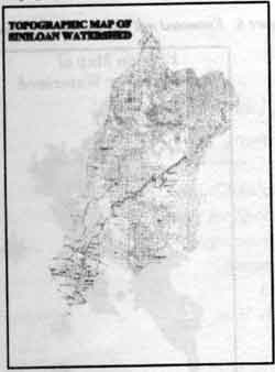
Figure 1. Topgraphic map of the watershed
Figure 1 present the Topographic map of the project area. The map looked as if it is manually mosaicked , cut and scanned. This was not the case, however. As explained in the Material and methods .The map is georeferenced, digitized and saved as vector geospatial data .
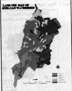
Figure 2. Land use map of the watershed.
Figure 2 showed the Land Use Map. Coconut and grasses are is the dominant land uses followed by forest .The other land uses are grasses and paddy rice.
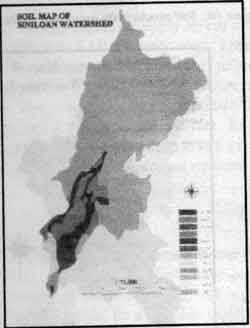
Figure 3.Soil map of the watershed.
Figure 3 is the soil map. Sampaloc series , slightly eroded is the dominant soil types in the upland area. For the low lands, the major soil are Coralan, Halayhayin , and Baybay series.
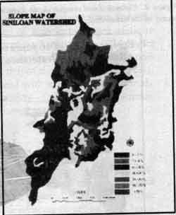
Figure 4 . Slope map of the watershed.
Figure 4 is the Slope Map. The lowlands are generally level (0-3% slope ). The sloping to undulating uplands have slopes of 3-18%. The complex mountain range that traverse the area has slopes of over 18%
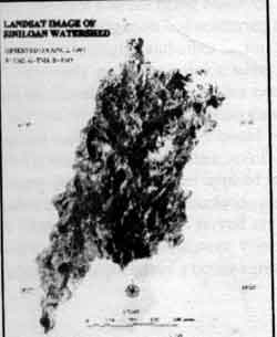
Figure 5.Landsat image of the watershed.
Figure 5 is the landsat Image of the watershed taken on Aril 2, 1993.
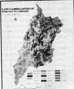
Figure 6. Land cover interpretation map based on landsat.
Figure 6 is the Land cover Interpretation Map of the Landsat image using the supervised classification function of TNTmips. The land cover map based on satellite image showed that coconut and grasses are the dominant vegetation in the area.
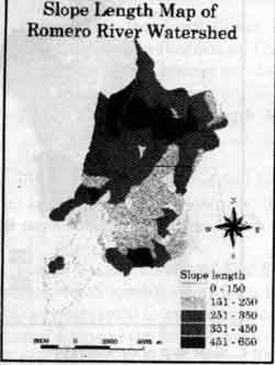
Figure 7. Slope length map of water shed.
Figure 7 is the slope Length Map of the watershed based on topographic and slope maps.
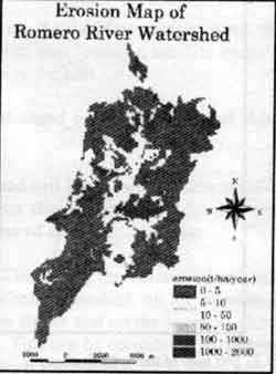
Figure 8 Estimated soil loss (tons/hectare/year)
Figure 8 is the Estimated Soil Loss Map. The estimated soil loss due to erosion is about 5 to 10 tons/ hectare /year. However, there are isolated areas that are suffering from severe erosion problems, with much as 100 to 1,000 tons/ hectare/year of soil loss.
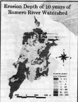
Figure 9. Estimated soil erosion depth (centimeters/10years) of the watershed.
Figure 9 is the Estimated Soil Erosion Depth Map. Converting the volume of soil loss into erosion depth (centimeters) for a ten year period, the whole watershed, on the average is not critically subjected to severe erosion hazard. Calculations shows that on the average, about 0.1 - 1 cm. Of topsoil can be lost due to erosion in ten years. This can be considered part of the natural soil renewal process. It can be noted that the GIS map identified critical areas where soil conservation is neede most. These are the areas where soil depth loss amount to 50 - 200 centimeters per ten years.
Summary and Conclusion
The following maps were prepared through GIS and remote sensing techniques as part of the development of geospatial database for the Romero River Watershed using TNT Map and image Processing System, PC ARCVIEW, and Fortran: (1) four thematic maps (topographic, land use, soil, slope), (2) three derived maps (land cover, slope length, soil productivity), and (3) two simulation model maps (soil loss in tons/ha/year and erosion depth in centimeters/10 years).
The computer-generated maps reveal critical areas of concern. Considering the Landsat image of the watershed vis-à-vis the depth of erosion estimates for the next ten years, it can be concluded that although agriculture is the dominant land use, the watershed analysis projected a minimal soil depth loss.
The combined GIS and remote sensing technology is an excellent tool for monitoring, land degradation, land use changes as well as soil and water resource changes over time.
In addition to the geospatial database report presentation and erosion studies, soil productivity studies as component of watershed analysis is being conducted to evaluate the soil dynamics. Figure 10 is the current Soil Productivity Capability Classification Rating Map of the watershed. The soil productivity rating of the different soil mapping units showed that in the lowlands the soils are class 1 or prime for rice. Still on-going is the study on given the erosion scenario (cm./per ten years), what would be the changes, if there be on the soil productivity ratin
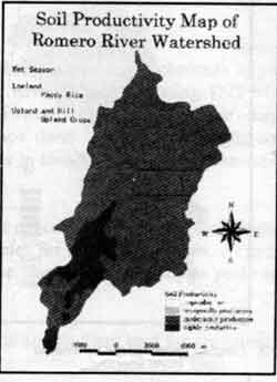
Figure 10. Soil productivity rating map of the watershed.