| GISdevelopment.net ---> AARS ---> ACRS 1997 ---> Poster Session 3 |
Mapping Seagrass From
Satellite Remote Sensing Data
Abd. Wahid Rasib and Mazlan
Hashim
Faculty of Engineering and Geoinformation Sciences
Universiti Teknologi Malaysia
Locked Bag 791, 80990 Johor Baharu
Tel : 07-5502969 Fax : 07-5566163,
Email : Mazlan@fksg.utm.my
Abstract Faculty of Engineering and Geoinformation Sciences
Universiti Teknologi Malaysia
Locked Bag 791, 80990 Johor Baharu
Tel : 07-5502969 Fax : 07-5566163,
Email : Mazlan@fksg.utm.my
This paper reviews some early results on a method adopted in mapping seagrass using Landsat-5 Thematic Mapper data. Seagrass information was extracted from satellite remotely sensed data using depth invariant index (DII) where the sea bottom features were expressed as index (i.e. each bottom type was represented by one index). DII was determined from radiance values recorded in band 1, 2 and 3 which taking into account the effect of water attenuation. Sea truth samples collected during the satellites overpass were used in calibrating DII and an independent accuracy assessment of information extracted.
Introduction
Remote sensing techniques have been used in various coastal marine applications. One of the applications in coastal/marine is for mapping shallow sea-bottom features by using Landsat TM data band 1 (0.45-0.52 mm), 2(0.52-0.60mm) and 3 (0.63-0.69mm). These data were accomplished with atmospheric correction which was effected referred by both Rayleigh and Aerosal path scatterings.
Material and Method
a) Study area
a) Study area covers an area of 14 400 Km2 situated in the coastal area of Penang Island and Langkawi Island, northwest of Peninsular Malaysia (see figure 1).
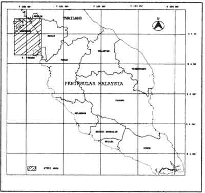
Figure 1. Location of the study area
b) Satellite data
The Landsat-5 TM data (path 126 and row 56) acquired on 11 March 95 at 2h 41 m 00 s UT were used in this study. Sea truth information at near realtime the satellite data acquisition were gathered from a selected transect at Telok Ewa, Langkawi Island.
c) Data processing
i) Atmospheric correction
Algorithm introduced by Sturm (1981b) was used to rectify the image affected by the atmospheric components such as Aerosol component and Rayleigh component. Both these corrections are given as :
TpA(l) = E (d,l). Toz(l,m,mo). ia(l).[PA(j)] + (r(l,m )+ (r(l,m0) PA(j+)]/cosq (2.0)
Where
TpR(l),TpA(l) are Rayleigh and Aerosol components, respectively
E (d,l) is the solar spectral irradiance
Toz(l,m,mo) is the beam transmittance ozone
ir(l, ia(l) are optic thickness of Rayleigh and Aerosol components
[PR(j+)],[PA(j+)] are function of phase of Rayleigh and Aerosol components
(r(l,m), (r(l,m0) are values of Freshnel reflectance
q is the sun zenith angle
ii) Geometric correction
The image was geometrically corrected where it is registered to Rectified Skew Orthomorphic Coordinate - map projection used for natural topographic mapping in Peninsular Malaysia.
iii) Extraction of seagrass
In short, figure 2 illustrates the extraction of subtrate reflectance over a water covered body. The light entering a water column is subjected to absorption and scattering from both the water body, and the light reflected back to the satellite is the main entity sought to extract sea bottom features.
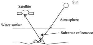
Figure 2. Illustration of substrate reflectance. Modified after Bierwirth (1993)
The relationship of reflectance recorded by satellite data and substrate reflectance, can be simplified (after Bierwirth, 1993) as :
Where
Dn is digital number
Ki is attenuatin coefficient for the water body.
-RB is the index substrate reflectance (radiance and water depth)
To determine Ki, the method adopted by Lyzenga (1981) was used where two bands were needed, such that ;
Where
Yi is value of known substrate reflectance
Li, Lj are radiance measured from band I and band j
Lsi , Lsj are radiance from deep area in band I and j
Ki, Kj are water attention coefficient irradiance for band i and band j
Results
The substrate reflectances or the depth invariant index (DII) computed using the first two TM bands is shown in figure 3. Sea-truth samples collected during satellite overpass were used to calibrate the DII. Using the pseudo color image transformation the sea-bottom feature map is produced (figure 4). A line map representing the sea-bottom features were then produced (figure 5).
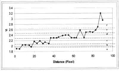
Figure 3. Classifications of sea bottom features using sea-truth samples.
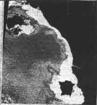
Figure 4. Pseudo color image showing the location and type of sea bottom features where seagrass is shown in shade of red.
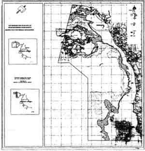
Figure 5. Final seagrass map- line map which is readily input to GIS
where
a and f are unknown layers
b is coarse sand
c is fine sand
d is mud
e is seagrass
Summary
In this study, remote sensing technique for mapping shallow-water bottom features namely seagrass has been presented. As this information is semi-dynamic, remote sensing techniques forms one of the best methods that can report the distribution of seagrass over large area, at economical rate.
References
- Lyzenga, D. R., (1981), "Remote Sensing of Bottom Reflectance And
WaterAttenuation Parameters". International Journal of Remote Sensing,
vol 2, no 1, pg 71-82.
- P. N. Bierwirth, T. J. Lee, R. V. Burne, (1993). "Shalow Sea-Floor
Reflectance and Water Depth Derived by Unmixing multispectral Imagery ".
Photogrammetric Engineering & Remote Sensing, vol. 59, No. 3, March,
pg 331-338.
- Sturm B., (1981b), " The Atmospheric Correction of Remotely Sensed
Data and the Quantitative Determination of Suspended Matter in Marine
Water Surface Layers. In Remote Sensing in meteorology, Oceanography and
Hydrology ", Edited by A. P. Cracknell, Halsted Press, ScotlandHalsted
Press,
Scotland.