| GISdevelopment.net ---> AARS ---> ACRS 1997 ---> Poster Session 3 |
Soil Nutrient Depletin
Modelling using Remote Sensig and GIS: A Case Study in Chonburi,
Thailand
Soe Win Myint1,
Chakkrit Thongthap2 and Dr. Apisit
Eiumnoh3
1UNEP Environment Assessment Program for Asia and the Pacific
Tel: 66-2 5246238, Fax : 662 5246233,
Email : swamyint@ait.ac.th
2Space Technology Application and Research Program
Tel: 66-2-52445584 , Fax" 662 52445597,
Email: nrd48826@ait.ac.th
AIT, P. O. Box 4, Klong Luang 12120 Thailand
Abstract1UNEP Environment Assessment Program for Asia and the Pacific
Tel: 66-2 5246238, Fax : 662 5246233,
Email : swamyint@ait.ac.th
2Space Technology Application and Research Program
Tel: 66-2-52445584 , Fax" 662 52445597,
Email: nrd48826@ait.ac.th
AIT, P. O. Box 4, Klong Luang 12120 Thailand
In this study soil nutrient depletion modeling of 3 major agricultural crop areas in Chonburi province were undertaken. Total N storage, and nutrient removal by crop and by soil less for a particular year are considered for this study. Land use map derived from TM acquired in 1995 was used in this study to identify cassava, paddy and sugarcane areas. Soil mass was obtained by calculating an area of a soil series, bulk density (BD) and an effective soil depth of a crop. As there is not direct measurement of N content in a soil system, organic carbon percent was used to calculate N amount in effective soil depth. The amount of P and K were obtained based on the available P and K value in PPM and soil mass in effective soil depth. N, P, and K taken up by tropical crops stated in UN-ESCAP, 1993 were used to compute the crop undertakes. Soil loss in the study area was obtained employing Universal Soil Loss Equation. A set of factors identified in USLE with several different approaches were reviewed, selected and applied, N, P, and K depletion due to soil erosion was obtained by the same method use for the availability of N, P, and K in a soil system by using organic carbon percent and P and K content from top 30 cm soil layer for all crops.
1. Introduction
The cause of nutrient depletion is due to the imbalance between the input and output of a soil system. Maintenance of proper nutrient status in soil is a key factor for high yield production. The inputs include nutrients in the soil profile, fertilizer application, nutrients derived from rainfall or from water apply to the crop, sediments accumulated on the soil and bio fixation. Nutrient removal from soil is due to uptake by crops, soil erosion, leaching, and volatization. The ability of soil to provide nutrients for crop production of fertility of a soil system is enhanced by systematic returns of nutrients. In order to properly manage nutrient balance of a soil system in a sustainable way it is necessary first to know availability, depletion and balance of nutrient in a soil system. This paper describes a study carried out to assess oil nutrient balance based on nutrient loss from two main sources: crop uptake and soil erosion. As far as possible other sources of nutrient input into the soil such as fertilizer use should be evaluated and included in the assessment of nutrient level. It seems that there is not much study and modeling for prediction of nutrient loss from leaching and volatization. Since the assessment of soil nutrient level, nutrient uptake by crops, and nutrient loss by soil erosion are very much related to spatial data GIS is a very effective tool in modeling nutrient status at various locations of a given study area. Spatial data used in this study includes land use/land cover, rainfall, soil characteristics (texture, depth, type, organic carbon percent, and Phosphorous and Potassium content of a soil system), topography (DEM, slope percent, slope length, and slope height), and nutrient uptake by crop for a unit area. Remote sensing is also required for preparing the land use/land cover map of an area for a given area for a give time. Since land use/land cover is a major factor in assessing nutrient depletion by crop uptakes and analyzing soil erosion, the importance of land use/land cover classification is obviously evident.
2. Study Area
This study area, Chonburi province of Thailand, is located between 100°50' N to 101° 43' and 12° 35' to 13° 36' in eastern part of Thailand. It has an area of 4,363.0 sq. km with population 977,000. Besides Forest, Rubber plantation and Mangrove major land use includes Paddy, cassava, sugarcane, pineapple, and orchard.
3. Materials and Supporting Data
Rainfall data (1995), Soil series map (1:100,000), Associates soil series information, Topographic map of Chonburi province (1:250,000), and Land use/land cover map of Chonburi Province derived from Landsat TM (1995) were used in this study.
4. Methodology
This study assumes that the nutrient uptakes by crops in a soil system is only from the nutrient in effective soil depth. The effective sol depth considered for cassava/sugarcane and paddy are 50 cm and 30 cm respectively. This can vary slightly due to the presence of hard rock, hard pan, water table and acid toxicity. Regarding nutrient loss from soil erosion, organic carbon percent, Phosphorous and Potassium in PPM (gm/ton) were taken from 30 cm soil depth. As the total nutrient loss was considered, the percentage of N available to plant was omitted in calculating nutrient loss from soil erosion. Soil loss assessment for the study area is based on the Universal Soil Loss Equation. Different calculation methods for each factor in Universal Soil Loss Equation were reviewed, selected and employed in this study. SLAMSA was also reviewed.
4.1 The Level of N, P, and K in Soil Series
From the soil series maps and associated soil series information organic carbon percent, Phosphorous and Potassium in PPM for respective soil depths were obtained.
4.1.1 Calculation of Available Nitrogen
There is not direct measurement about Nitrogen level in soils. Therefore, organic carbon percent was used to calculate the Nitrogen content in soil. From soil series map and associated description about soil series, information on organic carbon percent for each and every soil series from 30 cm soil depth for paddy and 50 cm soil depth for sugarcane and cassava were collected.Effective soil depth itself for each crop was also applied in obtaining soil mass. Nitrogen was given in the form of percentage of organic carbon which can be transferred in the form of organic matter by multiplication with the coefficient of 1.724. Five percent of total organic matter is estimated as Nitrogen content but only three percent of the total Nitrogen contained in matter is estimated as Nitrogen content but only three percent of the total Nitrogen contained in soil was computed as the weight of available Nitrogen which can be absorbed by crops. Bulk density in ton per cubic meter for each soil series was also obtained from soil series information. The calculation carried out for the availability of Nitrogen from a soil system is as follows:
| Total amount of soil mass(kg) | = area extent x soil depth x Bulk Density x 103 |
| The amount of organic matter (kg) | = soil mass x Organic Carbon % x 10-2 x 1.724 |
| The total of Nitrogen contained in a soil system (kg) | = organic matter content x 0.05 |
| The amount of Nitrogen available to plant (kg/ha) | = total Nitrogen x 0.03 x area extent of a 10-4 soil series in sq. m |
4.1.2 Calculation of Availbe Phosphorous
The content of phosphorous gram in one ton of soil expresses as PPM was obtained for paddy and sugarcane/cassava from 30 cm and 50 cm respectively. The Phosphorous and Potassium content vary from soil series to series. The calculation carried out for availability of Phosphorous is as follows:
| The amount of Phosphorous (kg) in 1 ha of soil | = (soil mass x P content / (area extent of a)) x 10 soil series in sq.m |
4.1.3 Calculation of Availabe Potassium
The same calculation process applied to obtain Phosphorous was also applied here.
4.2. Nutrient Removal by Crops
There were 20 land use and land cover classes derived form Landsat TM 1995. Only 3 main crop areas were included in this study. Usually three to five different sub classes were combined to form one big category. For instance, class no. 2 of paddy, class no. 18 of paddy plus orchard, class no. 24 of second rice, and class no. 25 of paddy plus plantation were merged as paddy. Effective soil depth is. The amount of nutrient up take by crop was identified and taken by the long-term experience of UN/ESCAP, 1993. N, P, and K removal by 3 main crops in kg from 1 ha of soil per year stated in UN/ESCAP, 1993 as follows:
| Paddy (total) | =N 219 | P31, | K258 | (kg/ha) |
| Cassava(total) | =N 120 | P40, | K187 | (kg/ha) |
| Sugarcane(total) | = N45, | P25, | K121 | (kg/ha) |
| Example: Nitrogen uptake by Paddy (kg)= Area extent of Paddy (sq.m)*10-4*219 | ||||
4.3 Nutrient Removal by Soil Erosion
Universal Soil Loss Equation (USLE, Wischmeier and Smith, 1965/1978) was applied in this study as which is by far the most widely used equation. Different approaches to obtain the factors influencing soil loss in USLE and Soil Loss Estimator for Southern Africa(SLAMSA, Elwell 1978a) were reviewed. Of all the approaches only the most suitable and appropriate methods for the factors in USLE were adopted in this study. Due to the lack of available data and information revised USLE (RUSLE, Renard et al., 1991), Water Erosion Prediction Project (WEPP, USDA, 1987), Chemicals, runoff, and erosion from agricultural management systems (CREAMS, Knisel, 1980), and Wind Erosion Prediction Equation (WEPE, Wood ruff and Siddoway 1965; Skidmore and Williams 1991) were omitted. Regarding RUSLE factor like prior land use which requires mass of live and dead roots and buried residues found in the upper 4 in and coefficient representing effectiveness of buried roots and residues information were not available. RUSLE requires a lot of field observation which are normally appropriate for a small watershed area. CREAMS, a combination of process-based and empirically based components, became widely used for field sized areas (Renard, et. al. 1995). In the case of WEPP sediment delivery estimates such as interill erodibility factor K are needed which is normally difficult to manage or not available for large areas. The WEPP is an effort to develop a technology for erosion prediction that extends into the next century (Foster and Land, 1987). WEPP's extensive data requirements and "block box" automated nature may limit its application in developing countries. Its precision and utility are as yet unproven, and its accuracy on steep slopes in the tropics is questionable (David E. Harper).
4.3.1 Calculations of Soil Loss using USLE
4.3.1.1 Rainfall Erosion Index (R )
The following 5 methods were reviewed and used to compute erosivity factor (R ). There were slight variations in all 5 equations.
| From Roose (1975), | |
| Mean annual rainfall erosion index (R ) in metric units | = 0.5 x P x 1.73 (1) |
| From Morgan (1974) | |
| Mean annual erosivity (MAE1) (KE>25) (j/m2) | = 9.28 x P - 8,838 |
| Multiply by I30 (75 mm/h; max. value recommended By Wischmeier) | = MAE1 x I30 (2) |
| From Foster el. al. (1981), | |
| Mean annual EI30 (MAE2) (kg.m.mm)/(m2.h) | = 0.276 x P x I30 |
| With these units, divide by 100 to give R value in Metric units | = MAE2/100 (3) |
| From Renard and Freimund, | |
| Rainfall erosion index (R ) in metric units | = 0.0048 x P1.61 (4) |
| From El-Swaify and others 1985, | |
| Rainfall erosion index (R ) in metric units | = 38.5 + 0.35 (P) (5) |
| From Wanapiryarat et. al. 1986, | |
| Daily erosivity factor in (y) | = -3.2353 + 1.789 ln (x) |
| Rainfall erosivity (index (R ) | = Sy (6) |
Where, P=Mean annual precipitation and x=Daily rainfall data. Results from equation 4 and 5 were found to be about average of all, the first one found to be the highest, and the second and third showed up the lowest. The results from the last equations were discarded and the average of the results from first three equations was taken as R-value in order to minimize the error. Since the rainfall data were not evenly distributed and not may measuring stations were situated in the study area, the calculated values in vector were converted to raster to provide polygon around a set of points.
4.3.1.2 Soil Erodibility Index (K)
K factor is combined effect of processes that regulate rainfall acceptance and the resistance of soil to particle detachment and subsequent transport. Here in this study the K values of different soil series were obtained by the method propose by Ahn, 1978. The approximate values of K were computed by comparing he percentages of clay, sand and silt contents of the soil with the triangular frame of reference provided by the author. The following is the formula developed by Wischmeir and Smith, 1978.
where, M = (% silt + % very fine sand) or (100-% clay), a = % of organic matter, b = soil structure class, and c = soil permeability class
4.3.1.3 Topographic Factor (LS)
The combined two factors in USLE the slop length (L) and slope in percent or degree (S) are generally known as topographic factor. Four methods for calculating slope length factor were considered. The first one developed by Wischeier and Smith (1978), the second one developed by McCool, et. al. 1989, Moore and Wilson 1992), the third one by McCool, et. al. 1987), and the last one by SLEMSA, Elwell 1978a).
Where, x is the slope length (m) and s is the slope gradient in percent. N = 0.5 for
Slope > 5%, 0.4 for slope 3.5 to 4.5%, 0.3 fro slope l to 3.5%, and 0.2 for slope less than 1%.
LS = (l /22)m (16.8 Sinb + 0.5) for slopes ³9.0%, (2)
Where, L = slope length in meters, b = slope gradient in degrees, M = F / (l + F), and F = (Sinb / 0.0896) / (3Sin0.8b + 0.56)
Where, L = slope length in meters, and s = slope gradient in percent.
Where, l is the slope length (m) and s is the slope steepness in percent. Calculation of combined LS factors based on all those equations showed that the result from the second method gives the best results compared to the others, which give high values for steep slopes.
4.3.1.4 The Combined Cover and Soil Conservation Factor (CP)
Of the USLE factors, values for the support practice (P) factor are the most uncertain (Renard et. al.). As accurate P values is not available for the study area these two factors were treated as a combined CP factor. C factor values were obtained from the table described in Soil Erosion and Conservation (1995) by R. P. C. Morgan after Wishmeier and Smith (1978); Roose (1977); Singh, Babu and Chandra (1981); El-Swaify, Dangler and Armstrong (1982); Hashim and Wong (1988) and the table prepared by Morgan and Finney (1982). P values for USLE were also obtained from the table stated in R. P. C. Morgan's Soil and Conservation (1995) after Wischmeir and Smith (1978); Roose (1977); Chan (19811a).
4.3.2 Calculation of Soil Loss using Slemsa
Soil loss (Z) = K . X . C
Computing K;
Mean annual rainfall energy (E) = 9.28 P - 8,838
Soil erodibility (F) could be obtained from table established by SLEMSA.
Mean annual soil loss (t/ha) from a standard field plot
ln K = b ln E +a
where, a = 2.884-8.1209 F, b = 0. 4681 + 0.7663 F
Computing X; For unridged land X = LS = (ò L (0.76 + 0.53s + 0.0765 s2) 25.65
Computing C; Crop management factor C = (2.3 - 0.01i) / 30
To calculate i value the conditions in percent described in the Crop cover ratings table associated with the SLEMSA formula were multiplied with mean annual rainfall occurring in that season. The results from SLEMSA formula were found to be reasonable. It is similar to the result from USLE with carefully adjusted factor values. However, the result SLEMSA was omitted as it is especially developed for Africa and suitable for unridged land condition.
4.4 Nutient Deplemetion by Soil Erosion
The same procedures applied in the calculation of available Nitrogen, Phosphorous, and Potassium in a soil system were applied here. But the Nitrogen available to the plant (3%) was not included and the organic carbon percent, Phosphorous and Potassium in PPM were taken only from top 30 cm soil layer as far as erosion is concerned.
4.5 Nutrient Balance
The following formula was used to compute the balance of nutrient in a soil system.
Nutrient balance = Available Nitrogen - (Nutrient uptake by crop+ Nutrient loss by soil erosion)
Final nutrient balance maps for Nitrogen, Phosphorous, and Potassium were prepared separately with the classes which include deficit 0-25, 25-50, 50-75, 75-100, 125-150, 150-200, above 200 kg/ha and nutrient surplus. Nitrogen balance map is shown as an example in Figure 1.
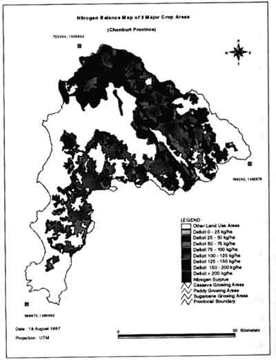
Figure 1.
5. Conclusion
High nutrient deficit especially of nitrogen is always associated with paddy and it indicates the need for Nitrogen application for such crop. But paddy has the least problem with Phosphorous. Sugarcane growing areas were found to be the least problem with nutrient depletion. The second highest nitrogen deficit is found to be associated with sugarcane. In general, the northern most pat of the province has the most serious problem with soil nutrient depletion. Since the techniques for nutrient depletion modeling have evolved only recently, limited study has been done in this regard and systematic study is still lacking. It is hoped that this study has been done in this regard and systematic study is still lacking. It is hoped that this study will be fulfilling such need. The study concluded that the techniques of integrating GIS and Remote Sensing for nutrient modeling are very much effective for assessing the nutrient status of a soil system for managing agriculture in a sustainable manner.
References
- ESCAP/FAO/UNIDO (1993). Balanced Fertilizer USE, It's a Practical Importance and Guidelines for Agriculture in the Asia-Pacific Region, H. L. S. Tandon (FDCO) and I. J. Kimmo (FADINAP).
- FAO/RAPA (1990). Problem soils of Asia and the Pacific, RAPA Report 1990/6, FAO Bangkok.
- Department of Land Development (1991). Soil Information System, (ISBN974-7696-83-5). DLD, Bangkok.
- FAO (1976). A framework for land evaluation, FAO Rome.
- National Research Council, the United States of America (1993). Soil and Water Quality, An Agenda for Agriculture, Committee on Long-range Soil and Water Conservation Board on Agriculture, Washington, D.C.
- Morgan, R. P. C. (1995). Soil Erosion and Conservation, Second Edition, Cranfield University, UK.
- Wischmeier, W. H. (1976). Use and Misuse of Universal Soil Loss Equaiton, Soil Science Society of America Proceedings, Vol. 31, No. 1, 5-9.
- Renard, K. G., Foster, G. R., Weesies, G. A., and Porter, J. P. (1991). RUSLE: Revised universal soil loss equation. Journal of Soil and Wate C onservation. 30-33.
- Renard, K. G., L. J. Lane, G. R. Foster, and J. M. Laflen (1993). Soil Loss Estimation, USDA. 170-201.
- Kok, K., Clavaux, M. B. W., Heerebout, W. M., and Bronsveld, K (1995). Land degradation and land cover change detection using low-resolution satellite images and the CORINE database: a case study in Spain. ITC Journal 1995-3. 217-228.
- Fook, L. K., Balhassan J., Mohmood N. N. (1992) Soil Erosion Mapping Using Remote Sensing and GIS Techniques for Land-Use Planners. ASIAN-PACIFIC Remote Sensing Journal, vol. 5, Number 1, July 1992 . 105-115.
- Euimnoh, A., Shrestha, R. P., Baimoung, S. (1996) Soil erosion assessment and its policy implications: A case study of RS and GIS applications in Uthai Thani, Thailand. Asian Conference on Remote Sensing, Proc. S-4-1 -S-4-6.